Content .. 193 194 195 196 ..

Physics For Scientists And Engineers 6E - part 195

SECTION 25.5 • Electric Potential Due to Continuous Charge Distributions

777

Example 25.8 Electric Potential Due to a Uniformly Charged Sphere

We can use this result and Equation 25.3 to evaluate the
potential difference V

at some interior point D:

# !

dr # !

r dr #

)

An insulating solid sphere of radius R has a uniform positive
volume charge density and total charge Q.

(A)

Find the electric potential at a point outside the sphere,

that is, for r . R. Take the potential to be zero at r # *.

Solution In Example 24.5, we found that the magnitude of
the electric field outside a uniformly charged sphere of
radius R is

where the field is directed radially outward when Q is posi-
tive. This is the same as the field due to a point charge,
which we studied in Section 23.4. In this case, to obtain the
electric potential at an exterior point, such as B in Figure
25.19, we use Equation 25.10, choosing point A as r # *:

(for r . R)

Because the potential must be continuous at r # R, we

can use this expression to obtain the potential at the surface
of the sphere. That is, the potential at a point such as C
shown in Figure 25.19 is

(B)

Find the potential at a point inside the sphere, that is,

for r & R.

Solution In Example 24.5 we found that the electric field
inside an insulating uniformly charged sphere is

(for r & R

)

(for r # R)

0 # k

(for r . R

)

constants, we find that

This integral has the following value (see Appendix B):

Evaluating V, we find

(25.25)

What If?

What if we were asked to find the electric field at

point P? Would this be a simple calculation?

V #

! )

√

)

(

√

)

(x )

√

)

V # k

√

)

√

)

Answer Calculating the electric field by means of Equation
23.11 would be a little messy. There is no symmetry to appeal
to, and the integration over the line of charge would repre-
sent a vector addition of electric fields at point P. Using
Equation 25.18, we could find E

by replacing a with y in

Equation  25.25  and  performing  the  differentiation  with
respect  to  y.  Because  the  charged  rod  in  Figure  25.18  lies
entirely  to  the  right  of  x # 0,  the  electric  field  at point  P
would have an x component to the left if the rod is charged
positively.  We  cannot  use  Equation  25.18  to  find the  x
component  of  the  field,  however,  because  we  evaluated  the
potential due to the rod at a specific value of x (x # 0) rather
than a general value of x. We would need to find the poten-
tial as a function of both x and y to be able to find the x and
y components of the electric field using Equation 25.25.

2
3

3 –

(

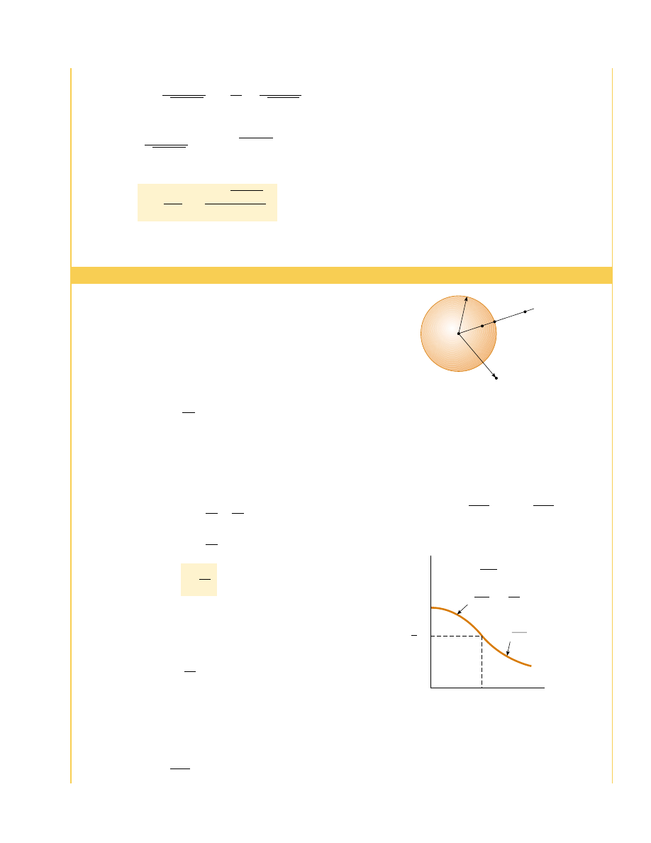
Figure 25.20 (Example 25.8) A plot of electric potential V

versus distance r from the center of a uniformly charged

insulating sphere of radius R. The curve for V

inside the

sphere is parabolic and joins smoothly with the curve for V

outside the sphere, which is a hyperbola. The potential has a

maximum value V

at the center of the sphere. We could make

this graph three dimensional (similar to Figures 25.8 and 25.9)

by revolving it around the vertical axis.

Figure 25.19 (Example 25.8) A uniformly charged insulating

sphere of radius R and total charge Q. The electric potentials at

points B and C are equivalent to those produced by a point

charge Q located at the center of the sphere, but this is not true

for point D.

25.6 Electric Potential Due to a Charged Conductor

In Section 24.4 we found that when a solid conductor in equilibrium carries a net
charge, the charge resides on the outer surface of the conductor. Furthermore, we
showed that the electric field just outside the conductor is perpendicular to the surface
and that the field inside is zero.

We now show that

every point on the surface of a charged conductor in equi-

librium is at the same electric potential. Consider two points A and B on the
surface of a charged conductor, as shown in Figure 25.21. Along a surface path
connecting these points,

E is always perpendicular to the displacement ds; therefore

E " ds # 0. Using this result and Equation 25.3, we conclude that the potential differ-
ence between A and B is necessarily zero:

This result applies to any two points on the surface. Therefore, V is constant every-
where on the surface of a charged conductor in equilibrium. That is,

# !

E"ds # 0

778

C H A P T E R 2 5 • Electric Potential

Substituting V

Q /R into this expression and solving

for V

, we obtain

(for r & R) (25.26)

3 !

(

At r # R, this expression gives a result that agrees with
that for the potential at the surface, that is, V

. A plot of

V versus r for this charge distribution is given in Figure
25.20.

+ + + +++

Figure 25.21 An arbitrarily shaped conductor carrying a positive

charge. When the conductor is in electrostatic equilibrium, all of

the charge resides at the surface, E # 0 inside the conductor, and

the direction of E just outside the conductor is perpendicular to

the surface. The electric potential is constant inside the conductor

and is equal to the potential at the surface. Note from the spacing

of the positive signs that the surface charge density is nonuniform.

the surface of any charged conductor in electrostatic equilibrium is an equipoten-
tial surface. Furthermore, because the electric field is zero inside the conductor, we
conclude that the electric potential is constant everywhere inside the conductor and
equal to its value at the surface.

Because this is true, no work is required to move a test charge from the interior of a
charged conductor to its surface.

Consider a solid metal conducting sphere of radius R and total positive charge Q ,

as shown in Figure 25.22a. The electric field outside the sphere is k

Q /r

and points

radially outward. From Example 25.8, we know that the electric potential at the
interior and surface of the sphere must be k

Q /R relative to infinity. The potential

outside the sphere is k

Q /r. Figure 25.22b is a plot of the electric potential as a

function of r, and Figure 25.22c shows how the electric field varies with r.

(a) +

(b)

(c)

Figure 25.22 (a) The excess

charge on a conducting sphere of

radius R is uniformly distributed on

its surface. (b) Electric potential

versus distance r from the center

of the charged conducting sphere.

distance r from the center of the

charged conducting sphere.

SECTION 25.6 • Electric Potential Due to a Charged Conductor

779

▲

PITFALL PREVENTION

25.6 Potential May Not

Be Zero

The  electric  potential  inside  the
conductor is not necessarily zero
in Figure 25.22, even though the
electric  field  is  zero.  From  Equa-
tion  25.15,  we  see  that  a  zero
value  of  the  field  results  in  no
change in  the  potential  from  one
point  to  another  inside  the  con-
ductor. Thus, the potential every-
where  inside  the  conductor,
including  the  surface,  has  the
same  value,  which  may  or  may
not be zero, depending on where
the  zero  of  potential  is  defined.

When a net charge is placed on a spherical conductor, the surface charge density

is uniform, as indicated in Figure 25.22a. However, if the conductor is nonspherical,
as in Figure 25.21, the surface charge density is high where the radius of curvature is
small (as noted in Section 24.4), and it is low where the radius of curvature is large.
Because the electric field just outside the conductor is proportional to the surface
charge density, we see that

the electric field is large near convex points having

small radii of curvature and reaches very high values at sharp points. This is
demonstrated in Figure 25.23, in which small pieces of thread suspended in oil show
the electric field lines. Notice that the density of field lines is highest at the sharp tip
of the left-hand conductor and at the highly curved ends of the right-hand conductor.
In Example 25.9, the relationship between electric field and radius of curvature is
explored mathematically.

Figure 25.24 shows the electric field lines around two spherical conductors: one

carrying a net charge Q , and a larger one carrying zero net charge. In this case, the
surface  charge  density  is  not  uniform  on  either  conductor.  The  sphere  having  zero
net charge has negative charges induced on its side that faces the charged sphere and
positive  charges  induced  on  its  side  opposite  the  charged  sphere.  The  broken  blue
curves in the figure represent the cross sections of the equipotential surfaces for this
charge  configuration.  As  usual,  the  field  lines  are  perpendicular  to  the  conducting
surfaces  at  all  points,  and  the  equipotential  surfaces  are  perpendicular  to  the  field
lines everywhere.

Figure 25.23 Electric field pattern

of a charged conducting plate

placed near an oppositely charged

pointed conductor. Small pieces of

thread suspended in oil align with

the electric field lines. The field

surrounding the pointed conduc-

tor is most intense near the

pointed end and at other places

where the radius of curvature is

small.

Q = 0

––

–

+
+

+++

+++++++

Figure 25.24 The electric field lines (in red-brown) around two spherical conductors.

The smaller sphere has a net charge Q , and the larger one has zero net charge. The

broken blue curves are intersections of equipotential surfaces with the page.

Quick Quiz 25.10

Consider starting at the center of the left-hand sphere

(sphere 1, of radius a) in Figure 25.24 and moving to the far right of the diagram, pass-
ing through the center of the right-hand sphere (sphere 2, of radius c) along the way.
The centers of the spheres are a distance b apart. Draw a graph of the electric potential
as a function of position relative to the center of the left-hand sphere.

Courtesy of Harold M. W

aage, Princeton University

A Cavity Within a Conductor

Now suppose a conductor of arbitrary shape contains a cavity as shown in Figure 25.26.
Let us assume that no charges are inside the cavity.

In this case, the electric field

inside the cavity must be zero regardless of the charge distribution on the outside
surface of the conductor. Furthermore, the field in the cavity is zero even if an electric
field exists outside the conductor.

To prove this point, we use the fact that every point on the conductor is at the same

electric potential, and therefore any two points A and B on the surface of the cavity
must be at the same potential. Now imagine that a field

E exists in the cavity and

evaluate the potential difference V

defined by Equation 25.3:

Because V

0, the integral of

E " ds must be zero for all paths between any two

points A and B on the conductor. The only way that this can be true for all paths is if

is zero everywhere in the cavity. Thus, we conclude that

a cavity surrounded by con-

ducting walls is a field-free region as long as no charges are inside the cavity.

Corona Discharge

A phenomenon known as

corona discharge is often observed near a conductor such

as a high-voltage power line. When the electric field in the vicinity of the conductor is
sufficiently strong, electrons resulting from random ionizations of air molecules near
the conductor accelerate away from their parent molecules. These rapidly moving
electrons can ionize additional molecules near the conductor, creating more free
electrons. The observed glow (or corona discharge) results from the recombination of

# !

E"d

780

C H A P T E R 2 5 • Electric Potential

Example 25.9 Two Connected Charged Spheres

Solution Because the spheres are connected by a conduct-
ing wire, they must both be at the same electric potential:

Therefore, the ratio of charges is

Because the spheres are very far apart and their surfaces
uniformly charged, we can express the magnitude of the
electric fields at their surfaces as

Taking the ratio of these two fields and making use of Equa-
tion (1), we find that

Hence, the field is more intense in the vicinity of the smaller
sphere even though the electric potentials of both spheres
are the same.

(2)

and

(1)

V # k

Two spherical conductors of radii r

and r

are separated by

a distance much greater than the radius of either sphere.
The spheres are connected by a conducting wire, as shown
in Figure 25.25. The charges on the spheres in equilibrium
are q

and q

, respectively, and they are uniformly charged.

Find the ratio of the magnitudes of the electric fields at the
surfaces of the spheres.

Figure 25.25 (Example 25.9) Two charged spherical conduc-

tors connected by a conducting wire. The spheres are at the

same electric potential V.

Figure 25.26 A conductor in elec-

trostatic equilibrium containing a

cavity. The electric field in the cav-

ity is zero, regardless of the charge

on the conductor.

Content .. 193 194 195 196 ..