Physics For Scientists And Engineers 6E - part 194

SECTION 25.4 •  Obtaining the Value of the Electric Field from the Electric Potential

773

If the charge distribution creating an electric field has spherical symmetry such that

the volume charge density depends only on the radial distance r, then the electric field
is  radial.  In  this  case, 

E " ds # E

r

dr,  and  we  can  express  dV in  the  form  dV # ! E

r

dr.

Therefore,

(25.17)

For example, the electric potential of a point charge is V # k

e

q/r. Because V is a func-

tion of r only, the potential function has spherical symmetry. Applying Equation 25.17,
we find that the electric field due to the point charge is E

r

#

k

e

q/r

2

, a familiar result.

Note  that  the  potential  changes  only  in  the  radial  direction,  not  in  any  direction
perpendicular to r. Thus, V (like E

r

) is a function only of r. Again, this is consistent with

the idea that 

equipotential surfaces are perpendicular to field lines. In this case

the  equipotential  surfaces  are  a  family  of  spheres  concentric  with  the  spherically
symmetric charge distribution (Fig. 25.13b).

The equipotential surfaces for an electric dipole are sketched in Figure 25.13c.
In  general,  the  electric  potential  is  a  function  of  all  three  spatial  coordinates.  If

V(r) is given in terms of the Cartesian coordinates, the electric field components E

x

, E

y

,

and E

z

can readily be found from V(x, y, z) as the partial derivatives

3

(25.18)

For example, if V # 3x

2

y ) y

2

)

yz, then

,

V

,

x

#

,

,

x

 

 (3x

 

2

y ) y

2

)

y

 

z) #

,

,

x

 

 (3x

 

2

y) # 3y 

  

d

dx

 

(x

 

2

) # 6x

 

y

E

x

# !

,

V

,

x

   

E

y

# !

,

V

,

y

   

E

z

# !

,

V

,

z

E

 

r

# !

dV

d

 

r

3

In vector notation, 

E is often written in Cartesian coordinate systems as

where - is called the gradient operator.

E # !-V # ! 

'

iˆ  

,

,

x

)

jˆ  

,

,

y

)

kˆ  

,

,

z

(

V

Quick  Quiz  25.8

In  a  certain  region  of  space,  the  electric  potential  is  zero

everywhere  along  the  x axis.  From  this  we  can  conclude  that  the  x component  of  the
electric field in this region is (a) zero (b) in the ) x direction (c) in the ! x direction.

Quick Quiz 25.9

In a certain region of space, the electric field is zero. From

this we can conclude that the electric potential in this region is (a) zero (b) constant
(c) positive (d) negative.

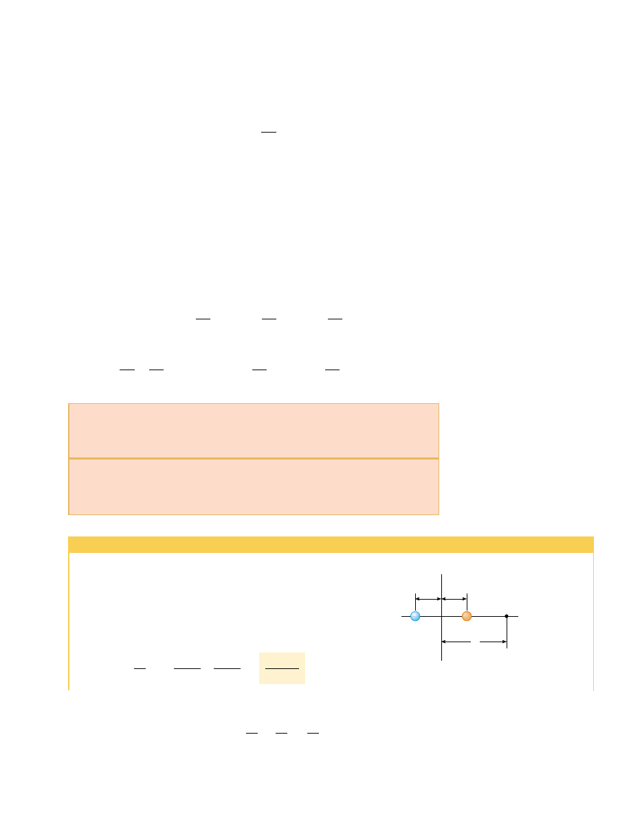
Example 25.4 The Electric Potential Due to a Dipole

An  electric  dipole  consists  of  two  charges  of  equal  magni-
tude and opposite sign separated by a distance 2a, as shown
in  Figure  25.14.  The  dipole  is  along  the  x axis  and  is
centered at the origin.

(A)

Calculate the electric potential at point P.

Solution For point P in Figure 25.14,

2k

e

  

qa

x

2

!

a

2

V # k

e  

&

 

 

q

 

i

r

i

#

k

e

  

 

'

q

x ! a

!

q

x ) a

(

#

a

a

q

P

x

x

y

–q

Figure 25.14 (Example 25.4) An electric dipole located on the

x axis.

Finding the electric field from

the potential

25.5 Electric Potential Due to Continuous

Charge Distributions

We  can  calculate  the  electric  potential  due  to  a  continuous  charge  distribution  in
two ways. If the charge distribution is known, we can start with Equation 25.11 for
the  electric  potential  of  a  point  charge.  We  then  consider  the  potential  due  to  a
small charge element dq, treating this element as a point charge (Fig. 25.15). The
electric potential dV at some point P due to the charge element dq is

(25.19)

where r is the distance from the charge element to point P. To obtain the total poten-
tial at point P, we integrate Equation 25.19 to include contributions from all elements
of  the  charge  distribution.  Because  each  element  is,  in  general,  a  different  distance
from point P and because k

e

is constant, we can express V as

(25.20)

In effect, we have replaced the sum in Equation 25.12 with an integral. Note that this
expression for V uses a particular reference: the electric potential is taken to be zero
when point P is infinitely far from the charge distribution.

If the electric field is already known from other considerations, such as Gauss’s law,

we can calculate the electric potential due to a continuous charge distribution using
Equation 25.3. If the charge distribution has sufficient symmetry, we first evaluate 

E at

any point using Gauss’s law and then substitute the value obtained into Equation 25.3
to determine the potential difference $V between any two points. We then choose the
electric potential V to be zero at some convenient point.

P R O B L E M - S O LV I N G   H I N T S

V # k

e

 

 

!

 

 

dq

r

dV # k

e

  

 

dq

r

774

C H A P T E R   2 5 •  Electric Potential

(B)

Calculate V and E

x

at a point far from the dipole.

Solution If point P is far from the dipole, such that x .. a,
then a

2

can be neglected in the term x

2

!

a

2

and V becomes

(x .. a)

Using  Equation  25.16  and  this  result,  we  can  calculate  the
magnitude  of  the  electric  field  at  a  point  far  from  the
dipole:

(x .. a)

(C)

Calculate  V and  E

x

if  point  P is  located  anywhere

between the two charges.

Solution Using Equation 25.12,

2

 

k

e

 

qx

a

 

2

!

x

 

2

V # k

e

 

  

&

 

 

q

 

i

r

i

#

k

e

  

 

'

q

a ! x

!

q

a ) x

(

#

4

 

k

e

 

qa

x

3

E

x

# !

dV

dx

#

V

)

2k

e

 

qa

x

 

2

We  can  check  these  results  by  considering  the  situation  at
the  center  of  the  dipole,  where  x # 0,  V # 0,  and
E

x

# !

2k

e

q/a

2

.

What  If?

What  if  point  P in  Figure  25.14  happens  to  be

located to the left of the negative charge? Would the answer
to part (A) be the same?

Answer The potential should be negative because a point
to the left of the dipole is closer to the negative charge than
to the positive charge. If we redo the calculation in part (A)
with P on the left side of ! q, we have

Thus,  the  potential  has  the  same  value  but  is  negative  for
points on the left of the dipole.

!

 

2

 

k

 

e

 

qa

x

2

!

a

2

V # k

e

 

  

&

 

 

q

 

i

r

i

#

k

e

  

 

'

q

x ) a

!

q

x ! a

(

#

r

P

dq

Figure 25.15 The electric poten-

tial at the point P due to a continu-

ous charge distribution can be

calculated by dividing the charge

distribution into elements of

charge dq and summing the

electric potential contributions

over all elements.

Electric potential due to a

continuous charge distribution

!

2

 

k

e

 

q

  

 

'

a

 

2

)

x

 

2

(a

 

2

!

x

 

2

)

2

(

E

x

# !

dV

dx

# !

d

dx

 

 

'

2

 

k

e

 

qx

a

 

2

!

x

 

2

(

#

and using Equation 25.16,

SECTION 25.5 •  Electric Potential Due to Continuous Charge Distributions

775

P R O B L E M - S O LV I N G   H I N T S

Calculating Electric Potential

•

Remember that electric potential is a scalar quantity, so vector components do
not exist. Therefore, when using the superposition principle to evaluate the
electric potential at a point due to a system of point charges, simply take the
algebraic sum of the potentials due to the various charges. However, you must
keep track of signs. The potential is positive for positive charges and negative
for negative charges.

•

Just as with gravitational potential energy in mechanics, only changes in electric
potential are significant; hence, the point where you choose the potential to be
zero is arbitrary. When dealing with point charges or a charge distribution of
finite size, we usually define V # 0 to be at a point infinitely far from the charges.

•

You can evaluate the electric potential at some point P due to a continuous
distribution of charge by dividing the charge distribution into infinitesimal
elements of charge dq located at a distance r from P. Then, treat one charge
element as a point charge, such that the potential at P due to the element is
dV # k

e

dq/r. Obtain the total potential at P by integrating dV over the entire

charge distribution. In performing the integration for most problems, you
must express dq and r in terms of a single variable. To simplify the integration,
consider the geometry involved in the problem carefully. Study Examples 25.5
through 25.7 below for guidance.

•

Another method that you can use to obtain the electric potential due to a finite
continuous charge distribution is to start with the definition of potential
difference given by Equation 25.3. If you know or can easily obtain 

E (from

Gauss’s law), then you can evaluate the line integral of 

E"ds. This method is

demonstrated in Example 25.8.

Example 25.5 Electric Potential Due to a Uniformly Charged Ring

than  a  set  of  discrete  charges,  we  categorize  this  problem
as one  in  which  we  need  to  use  the  integration  technique
represented by Equation 25.20. To analyze the problem, we
take point P to be at a distance x from the center of the ring,
as  shown  in  Figure  25.16.  The  charge  element  dq is  at  a 
distance 

from point P. Hence, we can express V as

Because each element dq is at the same distance from point P, 
we  can  bring 

in  front  of  the  integral  sign,  and  V

reduces to

(25.21)

The  only  variable  in  this  expression  for  V is  x.  This  is  not
surprising  because  our  calculation  is  valid  only  for  points
along the x axis, where y and z are both zero.

(B)

Find  an  expression  for  the  magnitude  of  the  electric

field at point P.

k

e

 

Q

√

x

 

2

)

a

 

2

V #

k

e

√

x

2

)

a

2

 

 

!

 dq #

√

x

 

2

)

a

 

2

V # k

e

 

  

!

 

dq

r

#

k

e

 

 

!

 

 

dq

√

x

 

2

)

a

 

2

 

√

x

 

2

)

a

 

2

(A)

Find an expression for the electric potential at a point

P located  on  the  perpendicular  central  axis  of  a  uniformly
charged ring of radius a and total charge Q.

Solution Figure 25.16, in which the ring is oriented so that
its plane is perpendicular to the x axis and its center is at the
origin,  helps  us  to  conceptualize  this  problem.  Because  the
ring  consists  of  a  continuous  distribution  of  charge  rather

P

x

√

x

2

 + a

2

dq

a

Figure 25.16 (Example 25.5) A uniformly charged ring of radius

a lies in a plane perpendicular to the x axis. All elements dq of the

ring are the same distance from a point P lying on the x axis.

776

C H A P T E R   2 5 •  Electric Potential

Solution From symmetry, we see that along the x axis 

E can

have only an x component. Therefore, we can use Equation
25.16:

 # !k

e

 

Q(!

1

2

)(x

 

2

)

a

 

2

)

!

3/2

 

(2x)

E

x

# !

d

 

V

d

 

x

# !

k

e

 

Q

   

 

d

dx

 

 (x

 

2

)

a

 

2

)

!

1/2

(25.22)

To  finalize  this  problem,  we  see  that  this  result  for  the
electric field agrees with that obtained by direct integration
(see Example 23.8). Note that E

x

#

0 at x # 0 (the center of

the ring). Could you have guessed this?

k

 

e

 

Qx

(x

 

2

)

a

 

2

)

3/2

E

x

#

Example 25.6 Electric Potential Due to a Uniformly Charged Disk

(25.23)

(B) As in Example 25.5, we can find the electric field at any
axial point using Equation 25.16:

(25.24)

The calculation of V and 

E for an arbitrary point off the axis

is more difficult to perform, and we do not treat this situa-
tion in this text.

2/k

e

  

 

0

  

'

1 !

x

√

x

2

)

a

2

(

E

x

# !

dV

dx

#

 2/k

e

 

 

0

  

[(x

 

2

)

a

 

2

)

1/2

!

x]

V #

A  uniformly  charged  disk  has  radius  a and  surface  charge
density 0. Find

(A)

the electric potential and

(B)

the magnitude of the electric field along the perpendic-

ular central axis of the disk.

Solution (A)  Again,  we  choose  the  point  P to  be  at  a
distance x from the center of the disk and take the plane of
the disk to be perpendicular to the x axis. We can simplify
the  problem  by  dividing  the  disk  into  a  series  of  charged
rings of infinitesimal width dr. The electric potential due to
each  ring  is  given  by  Equation  25.21.  Consider  one  such
ring of radius r and width dr, as indicated in Figure 25.17.
The  surface  area  of  the  ring  is  dA # 2/r dr.  From  the
definition  of  surface  charge  density  (see  Section  23.5),  we
know  that  the  charge  on  the  ring  is  dq # 0 dA # 02/r dr.
Hence, the potential at the point P due to this ring is

where  x is  a  constant  and  r is  a  variable.  To  find  the  total
electric potential at P, we sum over all rings making up the
disk. That is, we integrate dV from r # 0 to r # a:

This integral is of the common form 

and has the value

u

n+1

/(n ) 1), where n # ! and u # r

2

)

x

2

. This gives

1

2

*u

n

 

du

V # /

 

k

 

e

  

 

0

 

!

a

0

 

2r

  

d

 

r

√

r

2

)

x

2

#

/

 

k

 

e

  

 

0

  

 

!

a

0

 

 

(r

2

)

x

2

)

!

1/2

 2r

  

dr

dV #

k

e

 

dq

√

r

2

)

x

2

#

k

e

 

0

 

2/r dr

√

r

 

2

)

x

 

2

dr

dA = 2

π

rdr

√

r

2

 + x

2

x

P

r

a

π

Figure 25.17 (Example 25.6) A uniformly charged disk of

radius a lies in a plane perpendicular to the x axis. The calcula-

tion of the electric potential at any point P on the x axis is

simplified by dividing the disk into many rings of radius r and

width dr, with area 2

/

r dr.

Example 25.7 Electric Potential Due to a Finite Line of Charge

A rod of length ! located along the x axis has a total charge
Q and  a  uniform  linear  charge  density  1 # Q /!.  Find  the
electric potential at a point P located on the y axis a distance
a from the origin (Fig. 25.18).

Solution The  length  element  dx has  a  charge  dq # 1 dx.
Because  this  element  is  a  distance

from  point

P, we  can  express  the  potential  at  point  P due  to  this
element as

To obtain the total potential at  P, we integrate this expres-
sion over the limits x # 0 to x # !. Noting that k

e

and 1 are

dV # k

e

  

 

dq

r

#

k

e

  

 

1

 

 

dx

√

x

2

)

a

2

r #

√

x

 

2

)

a

 

2

dx

!

x

x

O

dq

r

a

P

y

Figure 25.18 (Example 25.7) A uniform line charge of length
!

located along the x axis. To calculate the electric potential at

P, the line charge is divided into segments each of length dx

and each carrying a charge dq #

1

dx.