Physics For Scientists And Engineers 6E - part 181

S E C T I O N   2 3 . 5 •  Electric Field of a Continuous Charge Distribution

721

total electric field at some point must be replaced by vector integrals. Divide
the charge distribution into infinitesimal pieces, and calculate the vector sum
by integrating over the entire charge distribution. Examples 23.7 through 23.9
demonstrate this technique.

•

Symmetry: with both distributions of point charges and continuous charge dis-
tributions, take advantage of any symmetry in the system to simplify your
calculations.

Example 23.7 The Electric Field Due to a Charged Rod

is particularly simple in this case. The total field at P due to all
segments of the rod, which are at different distances from P,
is given by Equation 23.11, which in this case becomes

3

where the limits on the integral extend from one end of the
rod (x ! a) to the other (x ! ! # a). The constants k

e

and 3

can be removed from the integral to yield

where we have used the fact that the total charge Q ! 3!.

What If?

Suppose we move to a point P very far away from

the rod. What is the nature of the electric field at such a point?

Answer If  P is  far  from  the  rod  (a -- !),  then  ! in  the
denominator of the final expression for E can be neglected,
and  E

" k

e

Q /a

2

.  This  is  just  the  form  you  would  expect

for a point  charge.  Therefore,  at  large  values  of  a/!,  the
charge distribution appears to be a point charge of magni-
tude Q —we are so far away from the rod that we cannot dis-
tinguish that it has a size. The use of the limiting technique
(

)  often  is  a  good  method  for  checking  a  mathe-

matical expression.

a/! : 4

k

e

 

Q

a(! # a)

!

k

e

 

 

3

 

&

1
a

"

1

! #

a

'

!

E ! k

e

 3

%

!#

a

a

 

dx
x

 

2

  ! k

e

 3 

(

"

1

x

)

a

!#

a

E !

%

!#

a

a

 k

e

 3 

dx
x

 

2

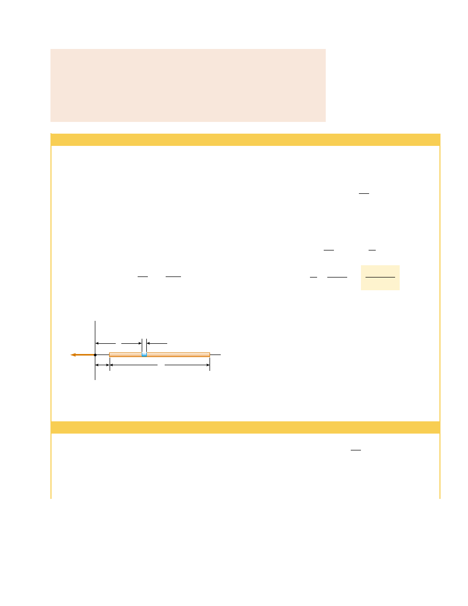
A  rod  of  length  ! has  a  uniform  positive  charge  per  unit
length 3 and a total charge Q. Calculate the electric field at
a point P that is located along the long axis of the rod and a
distance a from one end (Fig. 23.17).

Solution Let  us  assume  that  the  rod  is  lying  along  the
x axis, that dx is the length of one small segment, and that
dq is  the  charge  on  that  segment.  Because  the  rod  has  a
charge  per  unit  length  3,  the  charge  dq on  the  small
segment is dq ! 3 dx.

The field d

E at P due to this segment is in the negative

x direction (because the source of the field carries a positive
charge), and its magnitude is

Because every other element also produces a field in the neg-
ative x direction, the problem of summing their contributions

dE ! k

e 

 

dq
x

 

2

!

k

e 

 

3

 dx

x

 

2

3

It  is  important  that  you  understand  how  to  carry  out  integrations  such  as  this.  First,  express  the

charge element dq in terms of the other variables in the integral. (In this example, there is one vari-
able, x, and so we made the change dq ! 3 dx.) The integral must be over scalar quantities; therefore,
you must express the electric field in terms of components, if necessary. (In this example the field has
only an x component, so we do not bother with this detail.) Then, reduce your expression to an inte-
gral over a single variable (or to multiple integrals, each over a single variable). In examples that have
spherical or cylindrical symmetry, the single variable will be a radial coordinate.

x

y

!

a

P

x

dx

dq =

 

  

dx

E

3

Figure 23.17 (Example 23.7) The electric field at P due to a

uniformly charged rod lying along the x axis. The magnitude of

the field at P due to the segment of charge dq is k

e

dq/x

2

. The

total field at P is the vector sum over all segments of the rod.

This field has an x component dE

x

!

dE cos + along the x

axis and a component dE

⊥

perpendicular to the x axis. As

we  see  in  Figure  23.18b,  however,  the  resultant  field  at  P
must  lie  along  the  x axis  because  the  perpendicular  com-

d

 

E ! k

e 

 

dq
r

 

2

A  ring  of  radius  a carries  a  uniformly  distributed  positive
total charge Q. Calculate the electric field due to the ring at
a point P lying a distance x from its center along the central
axis perpendicular to the plane of the ring (Fig. 23.18a).

Solution The  magnitude  of  the  electric  field  at  P due  to
the segment of charge dq is

Example 23.8 The Electric Field of a Uniform Ring of Charge

722

C H A P T E R   2 3 •  Electric Fields

This  result  shows  that  the  field  is  zero  at  x =  0.  Does  this
finding surprise you?

What If?

Suppose a negative charge is placed at the center

of  the  ring  in  Figure  23.18  and  displaced  slightly  by  a
distance x !! a along the x axis. When released, what type of
motion does it exhibit?

Answer In  the  expression  for  the  field  due  to  a  ring  of
charge, we let x 55 a, which results in

Thus, from Equation 23.8, the force on a charge " q placed
near the center of the ring is

Because this force has the form of Hooke’s law (Eq. 15.1),
the motion will be simple harmonic!

F

x

! "

k

e

 

qQ

a

3

 x

E

x

!

k

e

 

Q

a

3

 x

ponents  of  all  the  various  charge  segments  sum  to  zero.
That is, the perpendicular component of the field created
by  any  charge  element  is  canceled  by  the  perpendicular
component created by an element on the opposite side of
the ring. Because r ! (x

2

#

a

2

)

1/2

and cos + ! x/r, we find

that

All  segments  of  the  ring  make  the  same  contribution
to the  field  at  P because  they  are  all  equidistant  from
this point. Thus, we can integrate to obtain the total field
at P:

k

e

 

x

(x

2

#

a

 

2

)

3/2

 

 

Q

!

E

x

!

%

 

k

e

 

x

(x

 

2

#

a

 

2

)

3/2

 

 dq !

k

e

 

x

(x

 

2

#

a

 

2

)

3/2

 

%

 dq 

d

 

E

x

!

d

 

E

 

cos + !

&

k

e 

 

dq
r

 

2

'

 

x

r

!

k

e

x

(x

2

#

a

2

)

3/2

 

 dq

(a)

+ +

+

+

+

+

+

+

+

+

+

+

+

+

+

+

θ

P

dE

x

dE

dE

⊥

x

r

dq

a

(b)

+ +

+

+

+

+

+

+

+

+

+

+

+

+

+

+

θ

dE

2

1

dE

1

2

Figure 23.18 (Example 23.8) A uniformly charged ring of radius a. (a) The field at P

on the x axis due to an element of charge dq. (b) The total electric field at P is along

the x axis. The perpendicular component of the field at P due to segment 1 is canceled

by the perpendicular component due to segment 2.

Example 23.9 The Electric Field of a Uniformly Charged Disk

A  disk  of  radius  R has  a  uniform  surface  charge  density  2.
Calculate  the  electric  field  at  a  point  P that  lies  along  the
central perpendicular axis of the disk and a distance x from
the center of the disk (Fig. 23.19).

Solution If we consider the disk as a set of concentric rings,
we can use our result from Example 23.8—which gives the
field  created  by  a  ring  of  radius  a—and  sum  the  contribu-
tions of all rings making up the disk. By symmetry, the field
at an axial point must be along the central axis.

The ring of radius r and width dr shown in Figure 23.19

has  a  surface  area  equal  to  2(r dr.  The  charge  dq on  this
ring is equal to the area of the ring multiplied by the surface
charge density: dq ! 2(2r dr. Using this result in the equa-
tion given for E

x

in Example 23.8 (with a replaced by r), we

have for the field due to the ring

d

 

E

x

!

k

e

 

x

(x

2

#

r

2

)

3/2

 

(2(2r dr)

To obtain the total field at P, we integrate this expression
over the limits r ! 0 to r ! R, noting that x is a constant.

P

x

r

R

dq

dr

Figure 23.19 (Example 23.9) A uniformly charged disk of ra-

dius R. The electric field at an axial point P is directed along

the central axis, perpendicular to the plane of the disk.

S E C T I O N   2 3 . 6 •  Electric Field Lines

723

This gives

2(k

e

 

2

 

 

&

1 "

x

(x

 

2

#

R

2

)

1/2

'

!

 

 ! k

e

 

x(2

 

 

(

(x

2

#

r

2

)

"

1/2

"

1/2

)

0

R

 

 ! k

e

 

x(2 

%

R

0

 (x

 

2

#

r

  

2

)

"

3/2

 d(r

 

 

2

)

E

x

 ! k

e

 

x(2 

%

R

0

 

2r dr

(x

2

#

r

2

)

3/2

This result is valid for all values of x - 0. We can calculate
the  field  close  to  the  disk  along  the  axis  by  assuming  that
R -- x ; thus, the expression in parentheses reduces to unity
to give us the near-field approximation:

where )

0 

is the permittivity of free space. In the next chapter

we  shall  obtain  the  same  result  for  the  field  created  by  a
uniformly charged infinite sheet. 

E

x

!

2(k

e

 

2 !

2

2)

0

23.6  Electric Field Lines

We have defined the electric field mathematically through Equation 23.7. We now explore
a  means  of  representing  the  electric  field  pictorially.  A  convenient  way  of  visualizing
electric field patterns is to draw curved lines that are parallel to the electric field vector at
any point in space. These lines, called electric field lines and first introduced by Faraday, are
related to the electric field in a region of space in the following manner:

• The  electric  field  vector 

E is tangent to the electric field line at each point. The

line  has  a  direction,  indicated  by  an  arrowhead,  that  is  the  same  as  that  of  the
electric field vector.

• The number of lines per unit area through a surface perpendicular to the lines is

proportional to the magnitude of the electric field in that region. Thus, the field
lines are close together where the electric field is strong and far apart where the
field is weak.

These  properties  are  illustrated  in  Figure  23.20.  The  density  of  lines  through

surface A is greater than the density of lines through surface B. Therefore, the magni-
tude of the electric field is larger on surface A than on surface B. Furthermore, the fact
that the lines at different locations point in different directions indicates that the field
is nonuniform.

Is  this  relationship  between  strength  of  the  electric  field  and  the  density  of  field

lines consistent with Equation 23.9, the expression we obtained for E using Coulomb’s
law? To answer this question, consider an imaginary spherical surface of radius r con-
centric with a point charge. From symmetry, we see that the magnitude of the electric
field is the same everywhere on the surface of the sphere. The number of lines N that
emerge from the charge is equal to the number that penetrate the spherical surface.
Hence, the number of lines per unit area on the sphere is N/4(r

2

(where the surface

area of the sphere is 4(

r

2

). Because E is proportional to the number of lines per unit

area, we see that E varies as 1/r

2

; this finding is consistent with Equation 23.9.

Representative electric field lines for the field due to a single positive point charge

are  shown  in  Figure  23.21a.  This  two-dimensional  drawing  shows  only  the  field  lines
that lie in the plane containing the point charge. The lines are actually directed radially
outward  from  the  charge  in  all  directions;  thus,  instead  of  the  flat  “wheel’’  of  lines
shown, you should picture an entire spherical distribution of lines. Because a positive
test charge placed in this field would be repelled by the positive source charge, the lines
are directed radially away from the source charge. The electric field lines representing
the  field  due  to  a  single  negative  point  charge  are  directed  toward  the  charge  (Fig.
23.21b). In either case, the lines are along the radial direction and extend all the way to
infinity. Note that the lines become closer together as they approach the charge; this in-
dicates that the strength of the field increases as we move toward the source charge.

B

A

Figure 23.20 Electric field lines

penetrating two surfaces. The mag-

nitude of the field is greater on sur-

face A than on surface B.

▲

PITFALL PREVENTION 

23.2 Electric Field Lines

are not Paths of
Particles!

Electric field lines represent the
field at various locations. Except
in very special cases, they do not
represent the path of a charged
particle moving in an electric
field.

724

C H A P T E R   2 3 •  Electric Fields

The rules for drawing electric field lines are as follows:

• The lines must begin on a positive charge and terminate on a negative charge.

In the case of an excess of one type of charge, some lines will begin or end infi-
nitely far away.

• The number of lines drawn leaving a positive charge or approaching a negative

charge is proportional to the magnitude of the charge.

• No two field lines can cross.

We choose the number of field lines starting from any positively charged object to

be  Cq and  the  number  of  lines  ending  on  any  negatively  charged  object  to  be  C

!q !,

where C is an arbitrary proportionality constant. Once C is chosen, the number of lines
is fixed. For example, if object 1 has charge Q

1

and object 2 has charge Q

2

, then the

ratio  of  number  of  lines  is  N

2

/N

1

!

Q

2

/Q

1

.  The  electric  field  lines  for  two  point

charges of equal magnitude but opposite signs (an electric dipole) are shown in Figure
23.22. Because the charges are of equal magnitude, the number of lines that begin at
the positive charge must equal the number that terminate at the negative charge. At
points  very  near  the  charges,  the  lines  are  nearly  radial.  The  high  density  of  lines
between the charges indicates a region of strong electric field.

(a)

+

–

▲

PITFALL PREVENTION 

23.3 Electric Field Lines

are not Real

Electric field lines are not mater-
ial objects. They are used only as
a  pictorial  representation  to
provide  a  qualitative  description
of the electric field. Only a finite
number  of  lines  from  each
charge  can  be  drawn,  which
makes  it  appear  as  if  the  field
were quantized and exists only in
certain  parts  of  space.  The  field,
in fact, is continuous—existing at
every point. You should avoid ob-
taining  the  wrong  impression
from  a  two-dimensional  drawing
of  field  lines  used  to  describe  a
three-dimensional situation.

(b)

Figure 23.22 (a) The electric field lines for two point charges of equal magnitude and

opposite sign (an electric dipole). The number of lines leaving the positive charge

equals the number terminating at the negative charge. (b) The dark lines are small

pieces of thread suspended in oil, which align with the electric field of a dipole. 

Courtesy of Harold M. W

aage, Princeton

University

(c)

(a)

q

(b)

–q

+

–

Figure 23.21 The electric field lines for a point charge. (a) For a positive point charge,

the lines are directed radially outward. (b) For a negative point charge, the lines are di-

rected radially inward. Note that the figures show only those field lines that lie in the

plane of the page. (c) The dark areas are small pieces of thread suspended in oil, which

align with the electric field produced by a small charged conductor at the center. 

Courtesy of Harold M. W

aage, Princeton University