Physics For Scientists And Engineers 6E - part 180

S E C T I O N   2 3 . 4 •  The Electric Field

717

direction as the field. If q is negative, the force and the field are in opposite directions.
Notice the similarity between Equation 23.8 and the corresponding equation for a par-
ticle with mass placed in a gravitational field, 

F

g

!

m

g (Eq. 5.6).

The vector 

E has the SI units of newtons per coulomb (N/C). The direction of E,

as shown in Figure 23.11, is the direction of the force a positive test charge experiences
when  placed  in  the  field.  We  say  that 

an  electric  field  exists  at  a  point  if  a  test

charge at that point experiences an electric force. Once the magnitude and direc-
tion  of  the  electric  field  are  known  at  some  point,  the  electric  force  exerted  on  any
charged  particle  placed  at  that  point  can  be  calculated  from  Equation  23.8.  The
electric field magnitudes for various field sources are given in Table 23.2.

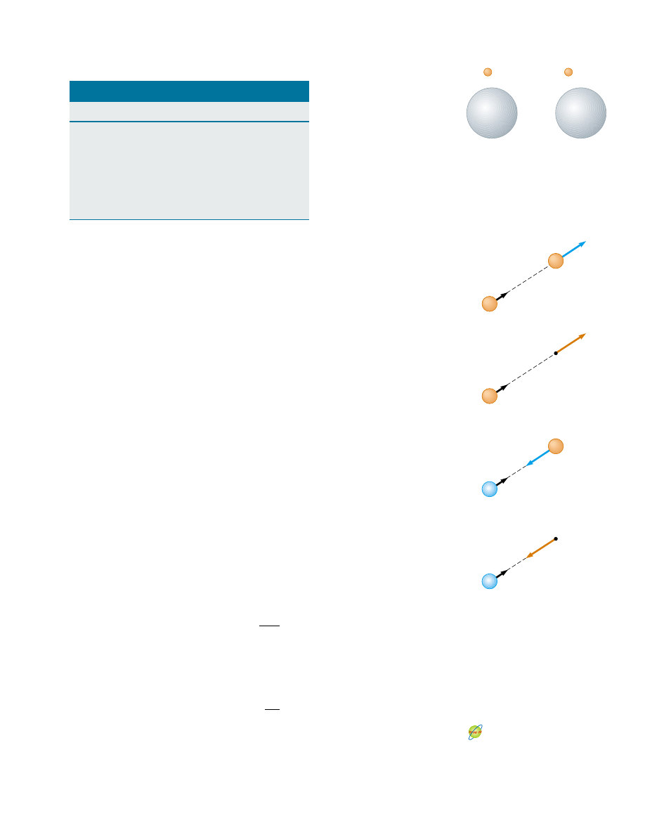
When using Equation 23.7, we must assume that the test charge q

0

is small enough

that it does not disturb the charge distribution responsible for the electric  field. If a
vanishingly small test charge q

0

is placed near a uniformly charged metallic sphere, as

in Figure 23.12a, the charge on the metallic sphere, which produces the electric field,
remains  uniformly  distributed.  If  the  test  charge  is  great  enough  (q

0

,

--

q

0

),  as  in

Figure 23.12b, the charge on the metallic sphere is redistributed and the ratio of the
force to the test charge is different: (F

e

,

/q

0

, .

F

e

/q

0

). That is, because of this redistribu-

tion of charge on the metallic sphere, the electric field it sets up is different from the
field it sets up in the presence of the much smaller test charge q

0

.

To  determine  the  direction  of  an  electric  field,  consider  a  point  charge  q as  a

source charge. This charge creates an electric field at all points in space surround-
ing it. A test charge q

0

is placed at point P, a distance r from the source charge, as in

Figure 23.13a. We imagine using the test charge to determine the direction of the
electric  force  and  therefore  that  of  the  electric  field.  However,  the  electric  field
does not depend on the existence of the test charge—it is established solely by the
source  charge.  According  to  Coulomb’s  law,  the  force  exerted  by  q on  the  test
charge is

where 

rˆ is  a  unit  vector  directed  from  q toward  q

0

.  This  force  in  Figure  23.13a  is

directed  away  from  the  source  charge  q.  Because  the  electric  field  at  P,  the  position
of the test charge, is defined by 

E ! F

e

/q

0

, we find that at P, the electric field created

by q is

(23.9)

If the source charge q is positive, Figure 23.13b shows the situation with the test charge
removed—the source charge sets up an electric field at point P, directed away from q.
If q is negative, as in Figure 23.13c, the force on the test charge is toward the source
charge,  so  the  electric  field  at  P is  directed  toward  the  source  charge,  as  in  Figure
23.13d.

E ! k

e

  

q

r

 

2

 

 

rˆ

 

F

e

!

k

e

  

qq

0

r

 

2

 

 

rˆ

Source

E (N/C)

Fluorescent lighting tube

10

Atmosphere (fair weather)

100

Balloon rubbed on hair

1 000

Atmosphere (under thundercloud)

10 000

Photocopier

100 000

Spark in air

-

3 000 000

Near electron in hydrogen atom

5 & 10

11

Typical Electric Field Values

Table 23.2

(a)

(b)

q

0

+

q

′

0

>>q

0

+

–

–

–

–

–

–

–

–

–

–

–

–

– –

–

–

–

–

–

–

–

–

–

–

Figure 23.12 (a) For a small

enough test charge q

0

, the charge

distribution on the sphere is undis-

turbed. (b) When the test charge

q

0

,

is greater, the charge distribu-

tion on the sphere is disturbed as

the result of the proximity of 

q

0

,

.

Active Figure 23.13 A test charge

q

0

at point P is a distance r from a

point charge q. (a) If q is positive,

then the force on the test charge is

directed away from q. (b) For the

positive source charge, the electric

field at P points radially outward

from q. (c) If q is negative, then the

force on the test charge is directed

toward q. (d) For the negative

source charge, the electric field at P

points radially inward toward q.

At the Active Figures link at

http://www.pse6.com, you can

move point P to any position in

two-dimensional space and 

observe the electric field due 

to q.

(b)

E

q

r

P

rˆ

+

(a)

F

q

q

0

r

P

rˆ

+

–

(c)

F

q

q

0

P

rˆ

–

(d)

E

q

P

rˆ

r

718

C H A P T E R   2 3 •  Electric Fields

To calculate the electric field at a point P due to a group of point charges, we first

calculate the electric field vectors at P individually using Equation 23.9 and then add
them vectorially. In other words,

at any point P, the total electric field due to a group of source charges equals the
vector sum of the electric fields of all the charges.

Quick Quiz 23.6

A test charge of # 3 *C is at a point P where an external

electric field is directed to the right and has a magnitude of 4 & 10

6

N/C. If the test

charge is replaced with another test charge of " 3 *C, the external electric field at P
(a) is unaffected (b) reverses direction (c) changes in a way that cannot be determined

Electric field due to a finite

number of point charges

Example 23.5 Electric Field Due to Two Charges

Solution First, let us find the magnitude of the electric field
at  P due  to  each  charge.  The  fields 

E

1

due  to  the  7.0-*C

charge  and 

E

2

due  to  the  " 5.0-*C  charge  are  shown  in

Figure 23.14. Their magnitudes are

The vector 

E

1

has only a y component. The vector 

E

2

has an

x component  given  by  E

2

cos + ! E

2

and  a  negative  y

component  given  by  " E

2

sin + ! " E

2

.  Hence,  we  can

express the vectors as

The resultant field 

E at P is the superposition of E

1

and 

E

2

:

From this result, we find that 

E makes an angle / of 66° with

the positive x axis and has a magnitude of 2.7 & 10

5

N/C.

(1.1 & 10

5

iˆ # 2.5 & 10

5

jˆ) N/C

E ! E

1

#

E

2

!

E

2

 ! (1.1 & 10

5

iˆ " 1.4 & 10

5

jˆ) N/C

E

1

 ! 3.9 & 10

5

jˆ  N/C

4

5

3

5

!

1.8 & 10

5

 N/C

E

2

!

k

e 

 

! q

 

2

!

r

 

2

 

2

!

(8.99 & 10

9

 N'm

2

/C

2

) 

(5.0 & 10

"

6

 C)

(0.50 m)

2

!

3.9 & 10

5

 N/C

E

1

!

k

e 

 

! q

 

1

!

r

 

1

 

2

!

(8.99 & 10

9

 N'm

2

/C

2

) 

(7.0 & 10

"

6

 C)

(0.40 m)

2

A charge q

1

!

7.0 *C is located at the origin, and a second

charge q

2

! "

5.0 *C is located on the x axis, 0.30 m from

the origin (Fig. 23.14). Find the electric field at the point P,
which has coordinates (0, 0.40) m.

0.40 m

P

θ

E

E

2

0.50 m

E

1

y

θ

x

q

2

q

1

0.30 m

–

φ

+

Figure 23.14 (Example 23.5) The total electric field E at P

equals the vector sum E

1

#

E

2

, where E

1

is the field due to the

positive charge q

1

and E

2

is the field due to the negative

charge q

2

.

This  superposition  principle  applied  to  fields  follows  directly  from  the  superposition
property  of  electric  forces,  which,  in  turn,  follows  from  the  fact  that  we  know  that
forces add as vectors from Chapter 5. Thus, the electric field at point P due to a group
of source charges can be expressed as the vector sum

(23.10)

where  r

i

is  the  distance  from  the  i th  source  charge  q

i

to  the  point  P and 

rˆ

i

is  a  unit

vector directed from q

i

toward P.

E ! k

e

 

 

$

 

i

q

i

r

i

2

 

 

rˆ

i

S E C T I O N   2 3 . 5 •  Electric Field of a Continuous Charge Distribution

719

The  y components  of 

E

1

and

E

2

cancel  each  other,  and

the x components are both in the positive x direction and
have  the  same  magnitude.  Therefore, 

E is parallel to the

x axis  and  has  a  magnitude  equal  to  2E

1

cos +.  From

Figure  23.15  we  see  that  cos + ! a/r ! a/(y

2

#

a

2

)

1/2

.

Therefore,

Because y -- a, we can neglect a

2

compared to y

2

and write

Thus,  we  see  that,  at  distances  far  from  a  dipole  but  along
the  perpendicular  bisector  of  the  line  joining  the  two
charges,  the  magnitude  of  the  electric  field  created  by  the
dipole varies as 1/r

3

, whereas the more slowly varying field

of  a  point  charge  varies  as  1/r

2

(see  Eq.  23.9).  This  is

because  at  distant  points,  the  fields  of  the  two  charges  of
equal  magnitude  and  opposite  sign  almost  cancel  each
other. The 1/r

3

variation in E for the dipole also is obtained

for a distant point along the x axis (see Problem 22) and for
any general distant point.

The  electric  dipole  is  a  good  model  of  many  mole-

cules, such as hydrochloric acid (HCl). Neutral atoms and
molecules  behave  as  dipoles  when  placed  in  an  external
electric field. Furthermore, many molecules, such as HCl,
are permanent dipoles. The effect of such dipoles on the
behavior  of  materials  subjected  to  electric  fields  is  dis-
cussed in Chapter 26.

k

e

 

 

2qa

y

 

3

E

"

 

!

k

e

 

 

2qa

(y

 

2

#

a

2

)

3/2

 E

 

!

2E

1

 cos + ! 2k

e 

 

q

(y

 

2

#

a

2

)

 

a

(y

 

2

#

a

2

)

1/2

An

electric  dipole  is  defined  as  a  positive  charge  q and  a

negative charge " q separated by a distance 2a. For the dipole
shown in Figure 23.15, find the electric field 

E at P due to the

dipole, where P is a distance y -- a from the origin.

Solution At P, the fields

E

1

and

E

2

due to the two charges

are  equal  in  magnitude  because  P is  equidistant  from  the
charges. The total field is 

E ! E

1

#

E

2

, where

E

1

!

E

2

!

k

e 

 

q

r

 

2

!

k

e 

 

q

y

2

#

a

2

Example 23.6 Electric Field of a Dipole

P

E

θ

θ

y

E

1

E

2

y

r

θ

a

q

θ

a

–q

–

x

+

Figure 23.15 (Example 23.6) The total electric field E at P due

to two charges of equal magnitude and opposite sign (an elec-

tric dipole) equals the vector sum E

1

#

E

2

. The field E

1

is due

to the positive charge q, and E

2

is the field due to the negative

charge " q.

23.5 Electric Field of a Continuous

Charge Distribution

Very often the distances between charges in a group of charges are much smaller than the
distance from the group to some point of interest (for example, a point where the electric
field is to be calculated). In such situations, the system of charges can be modeled as con-
tinuous. That is, the system of closely spaced charges is equivalent to a total charge that is
continuously distributed along some line, over some surface, or throughout some volume.

To evaluate the electric field created by a continuous charge distribution, we use the

following procedure: first, we divide the charge distribution into small elements, each of
which contains a small charge 0q, as shown in Figure 23.16. Next, we use Equation 23.9
to calculate the electric field due to one of these elements at a point P. Finally, we evalu-
ate the total electric field at P due to the charge distribution by summing the contribu-
tions of all the charge elements (that is, by applying the superposition principle).

The electric field at P due to one charge element carrying charge 0q is

0

E ! k

e 

 

0

q

r

 

2

 

 

rˆ

r

∆q

rˆ

P

∆E

Figure 23.16 The electric field at

P due to a continuous charge distri-

bution is the vector sum of the

fields 0E due to all the elements
0

q of the charge distribution.

where r is the distance from the charge element to point P and 

rˆ is a unit vector di-

rected from the element toward P. The total electric field at P due to all elements in
the charge distribution is approximately

where the index i refers to the i th element in the distribution. Because the charge dis-
tribution is modeled as continuous, the total field at P in the limit 0q

i

:

0 is

(23.11)

where the integration is over the entire charge distribution. This is a vector operation
and must be treated appropriately.

We illustrate this type of calculation with several examples, in which we assume the

charge is uniformly distributed on a line, on a surface, or throughout a volume. When
performing  such  calculations,  it  is  convenient  to  use  the  concept  of  a  charge  density
along with the following notations:

• If a charge Q is uniformly distributed throughout a volume V, the 

volume charge

density 1 is defined by

where 1 has units of coulombs per cubic meter (C/m

3

).

• If a charge Q is uniformly distributed on a surface of area A, the 

surface charge

density 2 (lowercase Greek sigma) is defined by

where 2 has units of coulombs per square meter (C/m

2

).

• If a charge Q is uniformly distributed along a line of length !, the 

linear charge

density 3 is defined by

where 3 has units of coulombs per meter (C/m).

• If  the  charge  is  nonuniformly  distributed  over  a  volume,  surface,  or  line,  the

amounts of charge dq in a small volume, surface, or length element are

dq ! 1 dV

dq ! 2 dA

dq ! 3 d!

3

 

# 

Q

!

2

 

# 

Q
A

1

 

# 

Q

V

E ! k

e

 

  lim

0

q

i

:

0

 

$

  

i

0

q

i

r

i

 

2

 

 

rˆ

i

!

k

e

 

%

 

dq

r

2

 

 

rˆ

E " k

e

 

 

$

 

i

0

q

i

r

i

 

2

 

 

rˆ

i

720

C H A P T E R   2 3 •  Electric Fields

P R O B L E M - S O LV I N G   H I N T S

Finding the Electric Field

•

Units: in calculations using the Coulomb constant k

e

(! 1/4()

0

), charges must

be expressed in coulombs and distances in meters.

•

Calculating the electric field of point charges: to find the total electric field at a
given point, first calculate the electric field at the point due to each individual
charge. The resultant field at the point is the vector sum of the fields due to
the individual charges.

•

Continuous charge distributions: when you are confronted with problems that
involve a continuous distribution of charge, the vector sums for evaluating the

Volume charge density

Surface charge density

Linear charge density

Electric field due to a

continuous charge distribution