Physics For Scientists And Engineers 6E - part 123

S E C T I O N   16 . 1 •  Propagation of a Disturbance

489

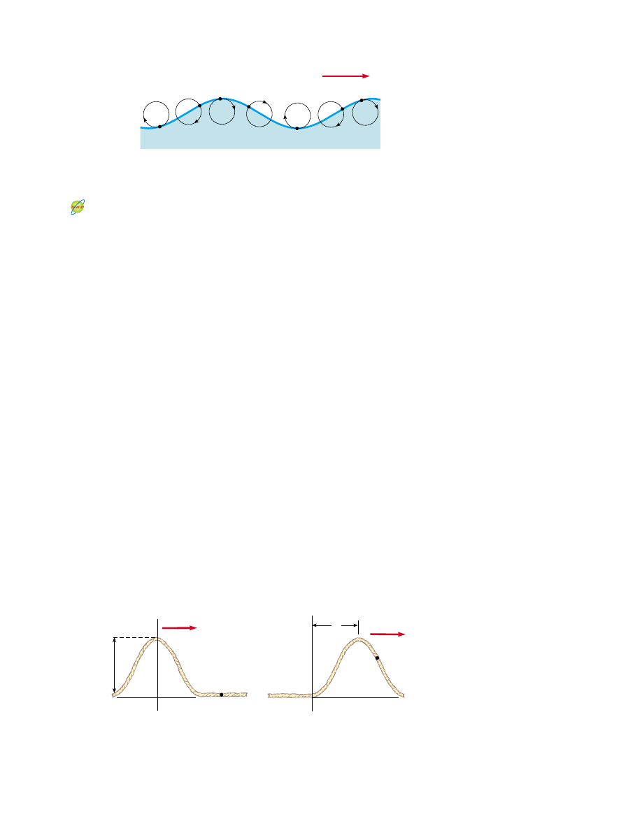
components. The transverse displacements seen in Figure 16.4 represent the variations
in  vertical  position  of  the  water  elements.  The  longitudinal  displacement  can  be  ex-
plained  as  follows:  as  the  wave  passes  over  the  water’s  surface,  water  elements  at  the
highest points move in the direction of propagation of the wave, whereas elements at
the lowest points move in the direction opposite the propagation.

The three-dimensional waves that travel out from points under the Earth’s surface

along a fault at which an earthquake occurs are of both types—transverse and longitu-
dinal. The longitudinal waves are the faster of the two, traveling at speeds in the range
of 7 to 8 km/s near the surface. These are called 

P waves (with “P” standing for pri-

mary) because they travel faster than the transverse waves and arrive at a seismograph
(a device used to detect waves due to earthquakes) first. The slower transverse waves,
called 

S  waves (with  “S”  standing  for  secondary),  travel  through  the  Earth  at  4  to  5

km/s near the surface. By recording the time interval between the arrivals of these two
types of waves at a seismograph, the distance from the seismograph to the point of ori-
gin  of  the  waves  can  be  determined.  A  single  measurement  establishes  an  imaginary
sphere centered on the seismograph, with the radius of the sphere determined by the
difference  in  arrival  times  of  the  P  and  S  waves.  The  origin  of  the  waves  is  located
somewhere on that sphere. The imaginary spheres from three or more monitoring sta-
tions located far apart from each other intersect at one region of the Earth, and this re-
gion is where the earthquake occurred.

Consider a pulse traveling to the right on a long string, as shown in Figure 16.5.

Figure 16.5a represents the shape and position of the pulse at time t ! 0. At this time,
the shape of the pulse, whatever it may be, can be represented by some mathematical
function  which  we  will  write  as  y(x,  0) ! f(x).  This  function  describes  the  transverse
position y of the element of the string located at each value of x at time t ! 0. Because
the speed of the pulse is v, the pulse has traveled to the right a distance vt at the time t
(Fig. 16.5b). We assume that the shape of the pulse does not change with time. Thus,
at time t, the shape of the pulse is the same as it was at time t ! 0, as in Figure 16.5a.

Active Figure 16.4 The motion of water elements on the surface of deep water in

which a wave is propagating is a combination of transverse and longitudinal displace-

ments, with the result that elements at the surface move in nearly circular paths. Each

element is displaced both horizontally and vertically from its equilibrium position.

Velocity of

propagation

A

y

(a) Pulse at  t = 0

O

vt

x

O

y

x

v

P

(b) Pulse at time t

P

v

Figure 16.5 A one-dimensional pulse traveling to the right with a speed v. (a) At t ! 0,

the shape of the pulse is given by y ! f (x). (b) At some later time t, the shape remains

unchanged and the vertical position of an element of the medium any point P is given

by y ! f (x " vt).

At the Active Figures link at http://www.pse6.com, you can observe the

displacement of water elements at the surface of the moving waves.

Consequently, an element of the string at x at this time has the same y position as an
element located at x " vt had at time t ! 0:

y(x, t) ! y(x " vt, 0)

In general, then, we can represent the transverse position y for all positions and times,
measured in a stationary frame with the origin at O, as

y(x, t) ! f (x " vt)

(16.1)

Similarly,  if  the  pulse  travels  to  the  left,  the  transverse  positions  of  elements  of  the
string are described by

y(x, t) ! f (x # vt)

(16.2)

The function y, sometimes called the 

wave function, depends on the two variables

x and t. For this reason, it is often written y(x, t), which is read “y as a function of x
and t.”

It is important to understand the meaning of y. Consider an element of the string

at  point  P,  identified  by  a  particular  value  of  its  x  coordinate.  As  the  pulse  passes
through P, the y coordinate of this element increases, reaches a maximum, and then
decreases  to  zero. 

The  wave  function  y(x,  t)  represents  the  y coordinate—the

transverse position—of any element located at position x at any time t. Further-
more, if t is fixed (as, for example, in the case of taking a snapshot of the pulse), then
the wave function y(x), sometimes called the 

waveform, defines a curve representing

the actual geometric shape of the pulse at that time.

490

C H A P T E R   16 •  Wave Motion

Pulse traveling to the right

A pulse moving to the right along the x axis is represented
by the wave function

where  x and  y are  measured  in  centimeters  and  t is  mea-
sured in seconds. Plot the wave function at t ! 0, t ! 1.0 s,
and t ! 2.0 s.

Solution First,  note  that  this  function  is  of  the  form
y ! f (x " vt).  By  inspection,  we  see  that  the  wave  speed  is
v ! 3.0 cm/s. Furthermore, the maximum value of y is given
by A ! 2.0 cm. (We find the maximum value of the function
representing  y by  letting  x " 3.0t ! 0.)  The  wave  function
expressions are

y(x, 1.0) !

2

(x " 3.0)

2

#

1

   

at t ! 1.0 s

y(x, 0) !

2

x

2

#

1

   

at t ! 0

y(x, t) !

2

(x " 3.0t)

2

#

1

We now use these expressions to plot the wave function ver-
sus x at these times. For example, let us evaluate y(x, 0) at
x ! 0.50 cm:

Likewise, at x ! 1.0 cm, y(1.0, 0) ! 1.0 cm, and at y ! 2.0 cm,
y(2.0, 0) ! 0.40 cm. Continuing this procedure for other val-
ues of x yields the wave function shown in Figure 16.6a. In a
similar manner, we obtain the graphs of y(x, 1.0) and y(x, 2.0),
shown  in  Figure  16.6b  and  c,  respectively.  These  snapshots
show  that  the  pulse  moves  to  the  right  without  changing  its
shape and that it has a constant speed of 3.0 cm/s.

What If?

(A)

What if the wave function were

y(x, t) !

2

(x # 3.0t)

2

#

1

y(0.50, 0) !

2

(0.50)

2

#

1

!

1.6 cm

y(x, 2.0) !

2

(x " 6.0)

2

#

1

   

at t ! 2.0 s

Pulse traveling to the left

Example 16.1 A Pulse Moving to the Right

Quick Quiz 16.1

In a long line of people waiting to buy tickets, the first per-

son leaves and a pulse of motion occurs as people step forward to fill the gap. As each
person steps forward, the gap moves through the line. Is the propagation of this gap
(a) transverse (b) longitudinal?

Quick Quiz 16.2

Consider the “wave” at a baseball game: people stand up

and shout as the wave arrives at their location, and the resultant pulse moves around
the stadium. Is this wave (a) transverse (b) longitudinal?

S E C T I O N   16 . 2 •  Sinusoidal Waves

491

Figure 16.6 (Example 16.1) Graphs of the function y(x, t) !

2/[(x " 3.0t)

2

#

1] at (a) t ! 0, (b) t ! 1.0 s, and (c) t ! 2.0 s.

y(cm)

2.0

1.5

1.0

0.5

0

1

2

3

4

5

6

y(x, 0)

t = 0

3.0 cm/s

(a)

x(cm)

y(cm)

2.0

1.5

1.0

0.5

0

1

2

3

4

5

6

y(x, 1.0)

t = 1.0 s

3.0 cm/s

(b)

x(cm)

y(cm)

2.0

1.5

1.0

0.5

0

1

2

3

4

5

6

y(x, 2.0)

t = 2.0 s

3.0 cm/s

(c)

x(cm)

7

7

8

How would this change the situation?

(B)

What if the wave function were

How would this change the situation?

y(x, t) !

4

(x " 3.0t)

2

#

1

Answer (A) The new feature in this expression is the plus
sign in the denominator rather than the minus sign. This re-
sults in a pulse with the same shape as that in Figure 16.6,
but moving to the left as time progresses.

(B) The new feature here is the numerator of 4 rather than
2. This results in a pulse moving to the right, but with twice
the height of that in Figure 16.6.

16.2 Sinusoidal Waves

In  this  section,  we  introduce  an  important  wave  function  whose  shape  is  shown  in
Figure 16.7. The wave represented by this curve is called a 

sinusoidal wave because

the curve is the same as that of the function sin $ plotted against $. On a rope, a sinu-
soidal wave could be established by shaking the end of the rope up and down in simple
harmonic motion.

The sinusoidal wave is the simplest example of a periodic continuous wave and can

be used to build more complex waves (see Section 18.8). The brown curve in Figure
16.7 represents a snapshot of a traveling sinusoidal wave at t ! 0, and the blue curve
represents a snapshot of the wave at some later time t. Notice two types of motion that
can be seen in your mind. First, the entire waveform in Figure 16.7 moves to the right,
so that the brown curve moves toward the right and eventually reaches the position of
the  blue  curve.  This  is  the  motion  of  the  wave.  If  we  focus  on  one  element  of  the
medium, such as the element at x ! 0, we see that each element moves up and down
along  the  y axis  in  simple  harmonic  motion.  This  is  the  motion  of  the  elements  of  the
medium. It is important to differentiate between the motion of the wave and the motion
of the elements of the medium.

Figure 16.8a shows a snapshot of a wave moving through a medium. Figure 16.8b

shows a graph of the position of one element of the medium as a function of time. The

t = 0

t

y

x

v

vt

Active Figure 16.7 A one-dimen-

sional sinusoidal wave traveling to

the right with a speed v. The brown

curve represents a snapshot of the

wave at t ! 0, and the blue curve

represents a snapshot at some later

time t.

At the Active Figures link

at http://www.pse6.com, you

can watch the wave move and

take snapshots of it at various

times.

point at which the displacement of the element from its normal position is highest is
called  the 

crest of  the  wave.  The  distance  from  one  crest  to  the  next  is  called  the

wavelength % (Greek lambda). More generally, the wavelength is the minimum dis-
tance between any two identical points (such as the crests) on adjacent waves, as
shown in Figure 16.8a.

If you count the number of seconds between the arrivals of two adjacent crests at a

given point in space, you are measuring the 

period T of the waves. In general, the pe-

riod is the time interval required for two identical points (such as the crests) of
adjacent waves to pass by a point. The period of the wave is the same as the period
of the simple harmonic oscillation of one element of the medium. 

The  same  information  is  more  often  given  by  the  inverse  of  the  period,  which  is

called the 

frequency f. In general, the frequency of a periodic wave is the number

of crests (or troughs, or any other point on the wave) that pass a given point in a
unit time interval. The frequency of a sinusoidal wave is related to the period by the
expression

(16.3)

The frequency of the wave is the same as the frequency of the simple harmonic oscilla-
tion  of  one  element  of  the  medium.  The  most  common  unit  for  frequency,  as  we
learned  in  Chapter  15,  is  second

"

1

,  or 

hertz (Hz).  The  corresponding  unit  for  T is 

seconds.

The  maximum  displacement  from  equilibrium  of  an  element  of  the  medium  is

called the 

amplitude A of the wave.

Waves travel with a specific speed, and this speed depends on the properties of the

medium being disturbed. For instance, sound waves travel through room-temperature
air with a speed of about 343 m/s (781 mi/h), whereas they travel through most solids
with a speed greater than 343 m/s.

Consider the sinusoidal wave in Figure 16.8a, which shows the position of the wave

at t ! 0. Because the wave is sinusoidal, we expect the wave function at this instant to
be expressed as y(x, 0) ! A sin ax, where A is the amplitude and a is a constant to be
determined.  At  x ! 0,  we  see  that  y(0,  0) ! A sin a(0) ! 0,  consistent  with  Figure
16.8a. The next value of x for which y is zero is x ! %/2. Thus,

For this to be true, we must have a(%/2) ! &, or a ! 2&/%. Thus, the function de-
scribing the positions of the elements of the medium through which the sinusoidal
wave is traveling can be written

(16.4)

where  the  constant  A represents  the  wave  amplitude  and  the  constant  % is  the  wave-
length.  We  see  that  the  vertical  position  of  an  element  of  the  medium  is  the  same
whenever x is increased by an integral multiple of %. If the wave moves to the right with
a speed v, then the wave function at some later time t is

(16.5)

That is, the traveling sinusoidal wave moves to the right a distance vt in the time t, as
shown in Figure 16.7. Note that the wave function has the form f (x " vt) (Eq. 16.1). If
the wave were traveling to the left, the quantity x " vt would be replaced by x # vt, as
we learned when we developed Equations 16.1 and 16.2.

y(x, t) ! A sin 

!

2&

%

 (x " vt)

"

y(x, 0) ! A sin 

#

2&

%

 

x

$

y 

#

%
2

, 0

$

!

A sin a 

#

%
2

$

!

0

f !

1

T

492

C H A P T E R   16 •  Wave Motion

Active Figure 16.8 (a) The wave-

length 

%

of a wave is the distance

between adjacent crests or adjacent

troughs. (b) The period T of a wave

is the time interval required for the

wave to travel one wavelength.

λ

y

λ

x

(a)

T

y

t

(b)

A

A

T

At the Active Figures link

at http://www.pse6.com, you

can change the parameters to

see the effect on the wave

function.

▲

PITFALL PREVENTION

16.1 What’s the

Difference Between
Figure 16.8a and
16.8b?

Notice  the  visual  similarity  be-
tween  Figures  16.8a  and  16.8b.
The  shapes  are  the  same,  but
(a) is a graph of vertical position
versus  horizontal  position  while
(b)  is  vertical  position  versus
time.  Figure  16.8a  is  a  pictorial
representation  of  the  wave  for  a
series  of  particles  of  the  medium—
this  is  what  you  would  see  at  an
instant  of  time.  Figure  16.8b  is  a
graphical  representation  of  the
position  of  one  element  of  the
medium as a function of time. The
fact  that  both  figures  have  the
identical  shape  represents  Equa-
tion  16.1—a  wave  is  the  same
function of both x and t.