Intel 64 and IA-32 Architectures. Software Developer’s Manual (Collection, 2023) - page 142

GENERAL OPTIMIZATION GUIDELINES
3.9.2.2
Dealing with Floating-Point Exceptions in x87 FPU Code
Every special situation listed in Section 3.9.2.1, “Floating-Point Exceptions,” is costly in terms of perfor-
mance. For that reason, x87 FPU code should be written to avoid these situations.
There are basically three ways to reduce the impact of overflow/underflow situations with x87 FPU code:
• Choose floating-point data types that are large enough to accommodate results without generating
arithmetic overflow and underflow exceptions.
• Scale the range of operands/results to reduce as much as possible the number of arithmetic
overflow/underflow situations.
• Keep intermediate results on the x87 FPU register stack until the final results have been computed
and stored in memory. Overflow or underflow is less likely to happen when intermediate results are
kept in the x87 FPU stack (this is because data on the stack is stored in double extended-precision
format and overflow/underflow conditions are detected accordingly).
• Denormalized floating-point constants (which are read-only, and hence never change) should be
avoided and replaced, if possible, with zeros of the same sign.
3.9.2.3
Floating-Point Exceptions in SSE/SSE2/SSE3 Code
Most special situations that involve masked floating-point exceptions are handled efficiently in hardware.
When a masked overflow exception occurs while executing Intel SSE/Intel SSE2/Intel SSE3/Intel
AVX/Intel AVX2/Intel AVX-512 code, processor hardware can handles it without performance penalty.
Underflow exceptions and denormalized source operands are usually treated according to the IEEE 754
specification1, but this can incur significant performance delay. If a programmer is willing to trade pure
IEEE 754 compliance for speed, two non-IEEE 754 compliant modes are provided to speed situations
where underflows and input are frequent: FTZ mode and DAZ mode.
When the FTZ mode is enabled, an underflow result is automatically converted to a zero with the correct
sign. Although this behavior is not compliant with IEEE 754, it is provided for use in applications where
performance is more important than IEEE 754 compliance. Since denormal results are not produced
when the FTZ mode is enabled, the only denormal floating-point numbers that can be encountered in FTZ
mode are the ones specified as constants (read only).
The DAZ mode is provided to handle denormal source operands efficiently when running a SIMD
floating-point application. When the DAZ mode is enabled, input denormals are treated as zeros with the
same sign. Enabling the DAZ mode is the way to deal with denormal floating-point constants when
performance is the objective.
If departing from the IEEE 754 specification is acceptable and performance is critical, run Intel SSE/Intel
SSE2/Intel SSE3/Intel AVX/Intel AVX2/Intel AVX-512 applications with FTZ and DAZ modes enabled.
NOTE
The DAZ mode is available with both the Intel SSE and Intel SSE2 extensions, although
the speed improvement expected from this mode is fully realized only in SSE code and
later.
3.9.3
Floating-Point Modes
For x87 code, using the FLDCW instruction to change floating modes can be an expensive operation in
many cases.
Recent processor generations provide hardware optimization for FLDCW that allows programmers to
alternate between two constant values efficiently. For the FLDCW optimization to be effective, the two
constant FCW values are only allowed to differ on the following 5 bits in the FCW:
1.
“IEEE Standard for Floating-Point Arithmetic,” in IEEE Std 754-2019 (Revision of IEEE 754-2008) , vol., no., pp.1-84, 22
July 2019, doi: 10.1109/IEEESTD.2019.8766229.
3-66

GENERAL OPTIMIZATION GUIDELINES
FCW[8-9]
; Precision control
FCW[10-11]
; Rounding control
FCW[12]
; Infinity control
If programmers need to modify other bits (for example: mask bits) in the FCW, the FLDCW instruction is
still an expensive operation.
In situations where an application cycles between three (or more) constant values, FLDCW optimization
does not apply, and the performance degradation occurs for each FLDCW instruction.
One solution to this problem is to choose two constant FCW values, take advantage of the optimization of
the FLDCW instruction to alternate between only these two constant FCW values, and devise some
means to accomplish the task that requires the 3rd FCW value without actually changing the FCW to a
third constant value. An alternative solution is to structure the code so that, for periods of time, the appli-
cation alternates between only two constant FCW values. When the application later alternates between
a pair of different FCW values, the performance degradation occurs only during the transition.
It is expected that SIMD applications are unlikely to alternate between FTZ and DAZ mode values.
Consequently, the SIMD control word does not have the short latencies that the floating-point control
register does. A read of the MXCSR register has a fairly long latency, and a write to the register is a seri-
alizing instruction.
There is no separate control word for single and double precision; both use the same modes. Notably,
this applies to both FTZ and DAZ modes.
Assembly/Compiler Coding Rule 52. (H impact, M generality) Minimize changes to bits 8-12 of
the floating-point control word. Changes for more than two values (each value being a combination of
the following bits: precision, rounding and infinity control, and the rest of bits in FCW) leads to delays
that are on the order of the pipeline depth.
3.9.3.1
Rounding Mode
Many libraries provide float-to-integer library routines that convert floating-point values to integer. Many
of these libraries conform to ANSI C coding standards which state that the rounding mode should be
truncation. With the Pentium 4 processor, one can use the CVTTSD2SI and CVTTSS2SI instructions to
convert operands with truncation without ever needing to change rounding modes. The cost savings of
using these instructions over the methods below is enough to justify using Intel SSE and Intel SSE2
wherever possible when truncation is involved.
For x87 floating-point, the FIST instruction uses the rounding mode represented in the floating-point
control word (FCW). The rounding mode is generally “round to nearest”, so many compiler writers imple-
ment a change in the rounding mode in the processor in order to conform to the C and FORTRAN stan-
dards. This implementation requires changing the control word on the processor using the FLDCW
instruction. For a change in the rounding, precision, and infinity bits, use the FSTCW instruction to store
the floating-point control word. Then use the FLDCW instruction to change the rounding mode to trunca-
tion.
In a typical code sequence that changes the rounding mode in the FCW, a FSTCW instruction is usually
followed by a load operation. The load operation from memory should be a 16-bit operand to prevent
store-forwarding problem. If the load operation on the previously-stored FCW word involves either an
8-bit or a 32-bit operand, this will cause a store-forwarding problem due to mismatch of the size of the
data between the store operation and the load operation.
To avoid store-forwarding problems, make sure that the write and read to the FCW are both 16-bit oper-
ations.
If there is more than one change to the rounding, precision, and infinity bits, and the rounding mode is
not important to the result, use the algorithm in Example 3-53 to avoid synchronization issues, the over-
head of the FLDCW instruction, and having to change the rounding mode. Note that the example suffers
3-67

GENERAL OPTIMIZATION GUIDELINES
from a store-forwarding problem which will lead to a performance penalty. However, its performance is
still better than changing the rounding, precision, and infinity bits among more than two values.
Example 3-53. Algorithm to Avoid Changing Rounding Mode
_fto132proc
lea
ecx, [esp-8]
sub
esp, 16
; Allocate frame
and
ecx, -8
; Align pointer on boundary of 8
fld
st(0)
; Duplicate FPU stack top
fistp
qword ptr[ecx]
fild
qword ptr[ecx]
mov
edx, [ecx+4]
; High DWORD of integer
mov
eax, [ecx]
; Low DWIRD of integer
test
eax, eax
je
integer_QnaN_or_zero
arg_is_not_integer_QnaN:
fsubp st(1), st
; TOS=d-round(d), { st(1) = st(1)-st & pop ST}
test
edx, edx
; What’s sign of integer
jns
positive
; Number is negative
fstp
dword ptr[ecx]
; Result of subtraction
mov
ecx, [ecx]
; DWORD of diff(single-precision)
add
esp, 16
xor
ecx, 80000000h
add
ecx,7fffffffh
; If diff<0 then decrement integer
adc
eax,0
; INC EAX (add CARRY flag)
ret
positive:
positive:
fstp
dword ptr[ecx]
; 17-18 result of subtraction
mov
ecx, [ecx]
; DWORD of diff(single precision)
add
esp, 16
add
ecx, 7fffffffh
; If diff<0 then decrement integer
sbb
eax, 0
; DEC EAX (subtract CARRY flag)
ret
integer_QnaN_or_zero:
test
edx, 7fffffffh
jnz
arg_is_not_integer_QnaN
add esp, 16
ret
Assembly/Compiler Coding Rule 53. (H impact, L generality) Minimize the number of changes to
the rounding mode. Do not use changes in the rounding mode to implement the floor and ceiling
functions if this involves a total of more than two values of the set of rounding, precision, and infinity
bits.
3.9.3.2
Precision
If single precision is adequate, use it instead of double precision. This is true because:
• Single precision operations allow the use of longer SIMD vectors, since more single precision data
elements can fit in a register.
• If the precision control (PC) field in the x87 FPU control word is set to single precision, the
floating-point divider can complete a single-precision computation much faster than either a
3-68

GENERAL OPTIMIZATION GUIDELINES
double-precision computation or an extended double-precision computation. If the PC field is set to
double precision, this will enable those x87 FPU operations on double-precision data to complete
faster than extended double-precision computation. These characteristics affect computations
including floating-point divide and square root.
Assembly/Compiler Coding Rule 54. (H impact, L generality) Minimize the number of changes to
the precision mode.
3.9.4
x87 vs. Scalar SIMD Floating-Point Trade-Offs
There are a number of differences between x87 floating-point code and scalar floating-point code (using
Intel SSE and Intel SSE2). The following differences should drive decisions about which registers and
instructions to use:
• When an input operand for a SIMD floating-point instruction contains values that are less than the
representable range of the data type, a denormal exception occurs. This causes a significant
performance penalty. An SIMD floating-point operation has a flush-to-zero mode in which the results
will not underflow. Therefore subsequent computation will not face the performance penalty of
handling denormal input operands. For example, in the case of 3D applications with low lighting
levels, using flush-to-zero mode can improve performance by as much as 50% for applications with
large numbers of underflows.
• Scalar floating-point SIMD instructions have lower latencies than equivalent x87 instructions. Scalar
SIMD floating-point multiply instruction may be pipelined, while x87 multiply instruction is not.
• Although x87 supports transcendental instructions, software library implementation of transcen-
dental function can be faster in many cases.
• x87 supports 80-bit precision, double extended floating-point. SSE support a maximum of 32-bit
precision. SSE2 supports a maximum of 64-bit precision.
• Scalar floating-point registers may be accessed directly, avoiding FXCH and top-of-stack restrictions.
• The cost of converting from floating-point to integer with truncation is significantly lower with Intel
SSE and Intel SSE2 in the processors based on Intel NetBurst microarchitecture than with either
changes to the rounding mode or the sequence prescribed in the Example 3-53.
Assembly/Compiler Coding Rule 55. (M impact, M generality) Use Streaming SIMD Extensions 2
or Streaming SIMD Extensions unless you need an x87 feature. Most SSE2 arithmetic operations have
shorter latency then their X87 counterpart and they eliminate the overhead associated with the
management of the X87 register stack.
3.9.4.1
Scalar Intel® SSE/Intel® SSE2
In code sequences that have conversions from floating-point to integer, divide single-precision instruc-
tions, or any precision change, x87 code generation from a compiler typically writes data to memory in
single-precision and reads it again in order to reduce precision. Using Intel SSE/Intel SSE2 scalar code
instead of x87 code can generate a large performance benefit using Intel NetBurst microarchitecture and
a modest benefit on Intel Core Solo and Intel Core Duo processors.
Recommendation: Use the compiler switch to generate scalar floating-point code using XMM rather
than x87 code.
When working with Intel SSE/Intel SSE2 scalar code, pay attention to the need for clearing the content
of unused slots in an XMM register and the associated performance impact. For example, loading data
from memory with MOVSS or MOVSD causes an extra micro-op for zeroing the upper part of the XMM
register.
3.9.4.2
Transcendental Functions
If an application needs to emulate math functions in software for performance or other reasons (see
Section 3.9.1, “Guidelines for Optimizing Floating-Point Code”), it may be worthwhile to inline math
3-69

GENERAL OPTIMIZATION GUIDELINES
library calls because the CALL and the prologue/epilogue involved with such calls can significantly affect
the latency of operations.
3.10
MAXIMIZING PCIE PERFORMANCE
PCIe performance can be dramatically impacted by the size and alignment of upstream reads and writes
(read and write transactions issued from a PCIe agent to the host’s memory). As a general rule, the best
performance, in terms of both bandwidth and latency, is obtained by aligning the start addresses of
upstream reads and writes on 64-byte boundaries and ensuring that the request size is a multiple of
64-bytes, with modest further increases in bandwidth when larger multiples (128, 192, 256 bytes) are
employed. In particular, a partial write will cause a delay for the following request (read or write).
A second rule is to avoid multiple concurrently outstanding accesses to a single cache line. This can result
in a conflict which in turn can cause serialization of accesses that would otherwise be pipelined, resulting
in higher latency and/or lower bandwidth. Patterns that violate this rule include sequential accesses
(reads or writes) that are not a multiple of 64-bytes, as well as explicit accesses to the same cache line
address. Overlapping requests—those with different start addresses but with request lengths that result
in overlap of the requests—can have the same effect. For example, a 96-byte read of address
0x00000200 followed by a 64-byte read of address 0x00000240 will cause a conflict—and a likely delay—
for the second read.
Upstream writes that are a multiple of 64-byte but are non-aligned will have the performance of a series
of partial and full sequential writes. For example, a write of length 128-byte to address 0x00000070 will
perform similarly to 3 sequential writes of lengths 16, 64, and 48 to addresses 0x00000070,
0x00000080, and 0x00000100, respectively.
For PCIe cards implementing multi-function devices, such as dual or quad port network interface cards
(NICs) or dual-GPU graphics cards, it is important to note that non-optimal behavior by one of those
devices can impact the bandwidth and/or latency observed by the other devices on that card. With
respect to the behavior described in this section, all traffic on a given PCIe port is treated as if it origi-
nated from a single device and function.
For the best PCIe bandwidth:
1. Align start addresses of upstream reads and writes on 64-byte boundaries.
2. Use read and write requests that are a multiple of 64-bytes.
3. Eliminate or avoid sequential and random partial line upstream writes.
4. Eliminate or avoid conflicting upstream reads, including sequential partial line reads.
Techniques for avoiding performance pitfalls include cache line aligning all descriptors and data buffers,
padding descriptors that are written upstream to 64-byte alignment, buffering incoming data to achieve
larger upstream write payloads, allocating data structures intended for sequential reading by the PCIe
device in such a way as to enable use of (multiple of) 64-byte reads. The negative impact of unoptimized
reads and writes depends on the specific workload and the microarchitecture on which the product is
based.
3.10.1 Optimizing PCIe Performance for Accesses Toward Coherent Memory and
MMIO Regions (P2P)
In order to maximize performance for PCIe devices in the processors listed in Table 3-7 the software
should determine whether the accesses are toward coherent (system) memory or toward MMIO regions
(P2P access to other devices). If the access is toward MMIO region, then software can command HW to
set the RO bit in the TLP header, as this would allow hardware to achieve maximum throughput for these
types of accesses. For accesses toward coherent memory, software can command HW to clear the RO bit
3-70

GENERAL OPTIMIZATION GUIDELINES
in the TLP header (no RO), as this would allow hardware to achieve maximum throughput for these types
of accesses.
Table 3-7. Intel Processor CPU RP Device IDs for Processors Optimizing PCIe Performance
Processor
CPU RP Device IDs
Intel® Xeon processors based on Broadwell microarchitecture
6F01H-6F0EH
Intel® Xeon processors based on Haswell microarchitecture
2F01H-2F0EH
3.11
SCALABILITY WITH CONTENDED LINE ACCESS IN 4TH GENERATION
INTEL® XEON® SCALABLE PROCESSORS
A two-socket system like that found in the Sapphire Rapids microarchitecture can have up to 224 (2
sockets x 56 cores/socket x 2 threads/core) hardware threads. Scalability and performance bottlenecks
may happen when all of these hardware threads compete for the same address.
3.11.1 Causes of Performance Bottlenecks
When multiple hardware threads go after the same address (for example, AA), this address is queued
in the Ingress Queue, with one entry for each hardware thread. Due to the resource limitation of the
Ingress Queue, the CPU core is throttled to slow the rate of requests when this queue overflows. This
usually occurs with contention for a lock.
3.11.2 Performance Bottleneck Detection
When multiple cores are contending on the same lock, several outstanding requests are mapped to that
same address. The Phys_addr_match event can count as such an event. This CHA event increments by
one every other cycle when there is more than one outstanding request to the same address.
Here are the PMU event id and Umask for the 2 CHA events that are very useful for detecting contention:
1. Phys_addr_match event:
Event id: 0x19, Umask: 0x80
2. CHA_clockticks event:
Event id: 0x01, Umask: 0x01
These events have to be measured on a per-CHA basis, and if the ratio of the counts between phys_ad-
dr_match to CHA_clockticks is more than 0.15 on any CHA that indicates > 30% of the CHA cycles (2x
the ratio as this event can count only once every two cycles) are spent with multiple requests outstanding
to the same address.
Here is the recipe to measure these events with Linux Perf:
$ sudo perf stat -a -e 'uncore_cha/event=0x19,umask=0x80/,uncore_cha/event=0x1,umask=0x1/' --per-socket
--no-merge -- sleep 30
Once confirmed that the ratio of phys_addr_match events to the CHA clockticks is more than 0.15, the
next step is figuring out where this may be happening in the code. Intel CPUs provide a PMU mechanism
wherein a load operation is randomly selected and tracked through completion, and the true latency is
recorded if it is over a given threshold. The threshold value is specified in cycles and must be in the power
of 2. In the following “perf mem record” command, define a command to sample all loads that take more
than 128 cycles to complete.
$ sudo perf mem record -a --ldlat 128 sleep 1
3-71

GENERAL OPTIMIZATION GUIDELINES
Once the above data is collected, execute the following command to process the data collected:
$ sudo perf mem report
Information similar to the table below will be generated. Such information will include details on hot loads
along with data linear address and the actual latency that the load experienced. This can be used to iden-
tify the necessary fixes to the code.
Table 3-8. Samples: 365K of Events ‘anon group{cpu/mem-loads-aux/,cpu/mem-loads,ldat=128/pp}’, Event Count (a--r0x):
67900852
0.22%
1
1
HitM
Yes
N/A
47251
0.07%
38060
0.18%
1
1
HitM
Yes
N/A
40411
0.06%
31338
0.17%
1
1
HitM
Yes
N/A
36652
0.06%
29572
3.11.3 Solutions for Performance Bottlenecks
The following is a list of suggested solutions:
1. Run multiple instances of the workload with a scale-out approach instead of a single instance
with scale-up so that the contention for per instance hot variables (including locks) is reduced.
2. Guard the cmpxchg by checking that the destination memory is expected with a load, test, and
branch beforehand.
3-72

GENERAL OPTIMIZATION GUIDELINES
3. Implement a backoff mechanism so that the cmpxchg is issued less. For example, in locks,
exponential backoff is a common and effective method to prevent all cores from being in
lockstep. In the case of contention for a lock, checking to see if it is accessible by a load before
trying to write to it through a cmpxchg will help.
The code in Example 3-54 provides an example:
Example 3-54. Locking Algorithm for the Sapphire Rapids Microarchitecture
lock_loop:
while (lock is not free) // just a load operation
execute pause;
// now the lock is free, so try to acquire it.
Exponential Backoff spin // so all the cores don’t come back at the same time
Execute cmpxchg on the lock
if the lock is not successfully acquired, goto lock_loop
Additionally, as the core counts continue to increase, exploring other algorithmic fixes that dissolve or
reduce contention on memory variables (including locks) is essential. For example, instead of frequently
updating a hot statistical variable from all threads, consider updating a copy of it per thread (without
contention) and later aggregate the updated per-thread copies on a less frequent basis or use some
existing atomic-free concurrency methods such as rseq1. As another example, restructure locking algo-
rithms to use hierarchical locking when excessive contention is detected on a global lock.
3.11.4 Case Study: SysBench/MariaDB Metric CHA % Cycles Fast Asserted
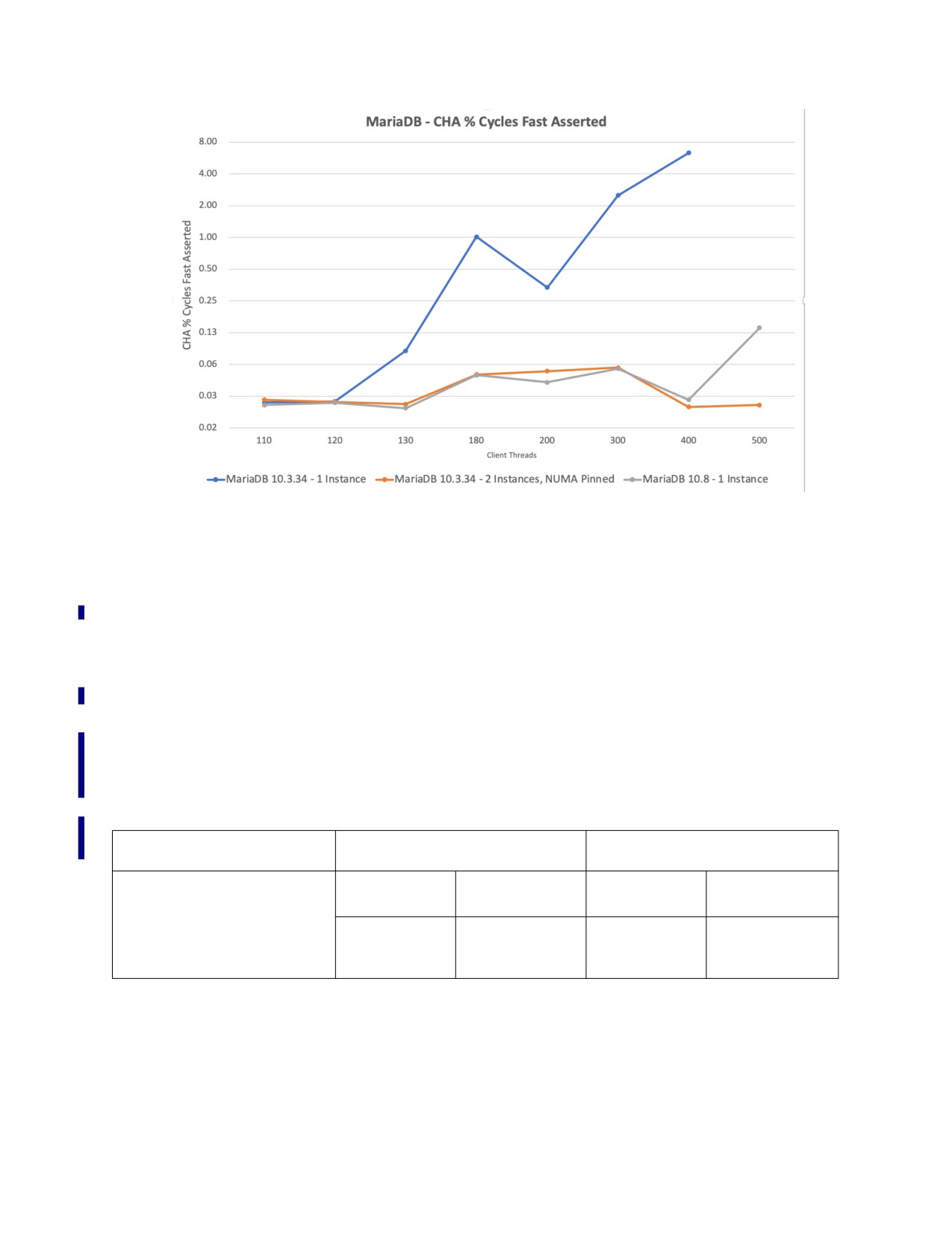
With SysBench/MariaDB 10.3.342, the workload’s throughput drops as the number of threads increases.
Another metric we can use is the CHA% Cycles Fast Asserted. It is a signal to slow down the cores when
the Ingress Queue fills up. This is another way to identify scalability issues. The graph below plots the
number of active client threads representing the work intensity on the horizontal axis. The percentage of
Fast Asserts is plotted on the vertical axis.
The baseline case (blue line) had a sharp throughput with increased thread count, as all cores reduced
their throughput as they suffered from the increasing percent of Fast Asserts. With the same work
distributed instances (red line), Fast asserts dropped. Similarly, with a software fix (gray line), again, the
Fast Asserts dropped even though only one instance was in execution.
1.
2. The most current version is MariaDB 10.3.39
3-73
GENERAL OPTIMIZATION GUIDELINES
Figure 3-4. MariaDB - CHA % Cycles Fast Asserted
3.11.5 Instruction Sequence Slowdowns
The Golden Cove CPU microarchitecture upon which the Sapphire Rapids microarchitecture is based has
increased the cost of mixing Legacy SSE and VEX without clearing the state of upper registers for power
efficiency reasons.
3.11.5.1 Causes of Instruction Sequence Slowdowns
The Golden Cove CPU microarchitecture eliminated some hardware speed paths for power efficiency and
replaced them with microcode. The instruction sequence in Table 3-9 mixes VEX and Legacy SSE. It has,
for example, higher core cycles than on the previous generation Sunny Cove CPU microarchitecture for
the Ice Lake version of the 3rd Generation of Intel® Xeon® Scalable processors. The higher core cycles
are due to the execution of additional micro-operations.
Table 3-9. Instruction Sequence Mixing VEX on the Sapphire Rapids and Ice Lake Server Microarchitectures
Ice lake Server Microarchitecture
Sapphire Rapids Microarchitecture
Intel Assembly Code Syntax
(Sunny Cove Cores)
(Golden Cove Cores)
Inst Retired
Core Cycles
Inst Retired
Core Cycles
VPXOR XMM3, XMM3, XMM3;
VEXTRACTI128 XMM3, YMM3, 1;
PXOR XMM3, XMM3
3.00
1
3.00
388.04
3-74

GENERAL OPTIMIZATION GUIDELINES
3.11.5.2 Detecting Instruction Sequence Slowdowns
The event ASSISTS.SSE_AVX_MIX can be used to determine if there are VEX to legacy SSE transitions.
The following Linux perf command-line can be used while the workload is running:
$ sudo perf stat -e 'assists.sse_avx_mix’1 <workload>
With the Intel® TMA (Topdown Methodology) (there is a metric called Mixing_Vectors which gives the
percentage of injected blend uops out of all the uops issued. Usually, a Mixing_Vectors metric over 5% is
worth investigating. You can find more details in Appendix B1 of the Optimizations Guide.
3.11.5.3 Fixing Instruction Sequence Slowdowns
The following is a list of suggested solutions:
1. When possible, use VEX-encoded instructions for all the SIMD instructions when possible.
2. Insert a VZEROUPPER to tell the hardware that the state of the higher registers is clean
between the VEX and the legacy SSE instructions. Often the best way to do this is to insert a
VZEROUPPER before returning from any function that uses VEX (that does not produce a VEX
register) and before any call to an unknown function.
VZEROUPPER was inserted in the code sequence below and there are no SSE_AVX_MIX assists. With
this change, the Core Cycles do not have a performance inversion relative to the previous generation.
Table 3-10. Fixed Instruction Sequence with Improved Performance on Sapphire Rapids Microarchitecture
Sapphire Rapids
Ice lake Microarchitecture
ASSISTS.SSE
Intel Assembly Code Syntax
Microarchitecture
(Sunny Cove Cores)
_AVX_MIX
(Golden Cove Cores)
VPXOR XMM3, XMM3, XMM3;
Inst Retired
Core Cycles
Inst Retired
Core Cycles
VEXTRACTI128 XMM3, YMM3, 1;
4.00
2.00
4.00
1.00
0
PXOR XMM3, XMM3
3.11.6 Misprediction for Branches >2GB
The Golden Cove CPU is a wider machine and might exhibit a higher Top-down Microarchitecture Analy-
sis (TMA) Bad Speculation percentage. See B.1.1 for additional information about TMA. Some sources
of Bad Speculation are branch prediction misses. In this case, however, Bad Speculation is due to the
wider machine and less efficient branch prediction for certain indirect branches.
3.11.6.1 Causes of Branch Misprediction >2GB
For a near absolute indirect JMP/CALL branch instruction (opcodes FF /4 and FF /2), the branch distance
(ADDR_TARGET - ADDR_BRANCH) affects the performance of the branch predictor. The branch predictor
uses fewer resources to predict the branch if its distance can be specified with a 32-bit signed displace-
ment (JMP/CALL imm32). If the distance is larger (>2GB), the predictor uses more resources to predict
the branch and performance may suffer.
3.11.6.2 Detecting Branch Mispredictions >2GB
You can use the Last Branch Record (LBR) to identify jumps greater than 2GB. The collection of perfor-
mance analysis tools based on perf on Linux supports this. The following is an example output from the
tool. It shows that 21% of the call/jumps of >2GB offset are mispredicted. The histogram of one of the
1. Using upstream perf. If OS doesn’t have support for the event use
cpu/event=0xc1,umask=0x10,name=assists_sse_avx_mix/
3-75

GENERAL OPTIMIZATION GUIDELINES
indirect branches at address 0x555555603664 shows that it is to one target and in a library. The profile
mask is to use LBR, and the duration is 10 seconds. It does a system-level profile.
% ./do.py profile --profile-mask=0x100 -s 10
count of indirect call/jump of >2GB offset: 93200
count of mispredicted indirect call/jump of >2GB offset: 19943
misprediction ratio for indirect branch at address 0x7ffff577eca4: 4.23%
misprediction ratio for indirect branch at address 0x5555556030c4: 32.23%
misprediction ratio for indirect branch at address 0x555555603664: 22.30%
misprediction ratio for indirect branch at address 0x555555603c24: 13.84%
…
indirect_0x555555603664 histogram:
0x7ffff7af2670: 50501 100.0%
Figure 3-5. Identifying >2GB Branches
3.11.6.3 Fixing Branch Mispredictions >2GB
Arrange the code so the jumps don’t span the >2GB range. This can be done through a variety of
approaches:
1. If possible, statically link all the libraries into the executable.
2. For .text to library code, use the Glibc environment variable LD_PREFER_MAP_32BIT_EXEC=1 to
restrict the addresses into the 4GB range.
3. For dynamically compiled code, keep it close to the .text address or copy the frequently called entries
into the dynamically compiled code address region. See the Google V8 Blog.
In a case study with WordPress/PHP running eight containers with and without the 2GB fix, the CPI and
performance scores improve by 6%.
Table 3-11. WordPress/PHP Case Study: With and Without a 2GB Fix for Branch Misprediction
WP4.2 / PHP7.4.29
WP4.2 / PHP7.4.29 -
2G FIX/
- NO FIX
2G FIX in Glibc
NO FIX
Workers
8c x 42
8c x 42
-
Cores Per socket
56
56
1.00
Config
Sockets
2
2
1.00
Total Cores
112
112
1.00
Total Thread Count
224
224
1.00
Throughput
1.00
1.06
1.06
Performance
CPI
1.12
1.05
0.96
Path Length
Instructions per Unit of Work
33,789,862.68
33,730,155.10
1.00
Cycles per
Cycles per Unit of Work
37,803,310.48
35,359,628.33
0.94
Transaction
3-76
GENERAL OPTIMIZATION GUIDELINES
3.12
OPTIMIZING COMMUNICATION WITH PCI DEVICES ON INTEL® 4TH
GENERATION INTEL® XEON® SCALABLE PROCESSORS
The Sapphire Rapids microarchitecture introduced a new set of instructions designed to optimize
communication between SW running on IA cores and PCI devices on the platform.
3.12.1 Signaling Devices with Direct Move
Most software-to-device interaction follows a producer-to-consumer relationship where the software
creates work for the device and then signals it to inform the device that work is available. Descriptor rings
are the ubiquitous pattern here and once descriptors are added to the ring, the signal (or “doorbell”)
consists of an update to the tail pointer register on the device. This is a write to an MMIO-mapped BAR
register.
Such writes tend to be relatively expensive operations -the latency to complete the write to the device is
high relative to the CPU operating speed. Since writes are ordered by default, this creates a bubble
during which subsequent writes cannot be drained from store buffers. Signaling can therefore affect
performance via store backpressure.
As a result, some software libraries avoid frequent signaling by batching relatively large quantities of
work descriptors with each doorbell update. However, this is not always possible, and it introduces
latency.
The Sapphire Rapids microarchitecture introduces “Direct Store” instructions to optimize signaling; there
are two instructions in the family:
• MOVDIRI: 4/8B direct store.
• MOVDIR64B: 64B atomic direct copy.
Direct Stores are weakly ordered (like non-temporal or USWC-mapped memory writes) regardless of the
underlying memory type (which is usually UC for MMIO-mapped locations). Since they do not order
subsequent writes the performance issue described above does not occur.
Since they are intended for signaling, direct stores will never combine with other stores to the same
address as can happen with non-temporal or USWC writes. Each write is guaranteed to occur as issued.
In the case of MOVDIR64B, the full 64B will be delivered as a single write to the device. This is the only
ISA that carries an architectural guarantee of >8B atomicity.
These instructions benefit from the fact that signaling use cases typically do not care if subsequent writes
are observed before the doorbell itself because the ordering is relaxed. However, since typically the door-
bell must not be observable before earlier writes (such writes are creating the work descriptors), SW
should insert a store fence immediately before the direct store.
Having a fence before the direct store does not normally limit performance- except when many direct
stores are issued. If there is an SFENCE before each, the fence on direct store N+1 imposes an order on
direct store N, which can remove some of the benefits. The guideline is to avoid this where possible. One
technique that may work if multiple doorbells to different addresses are being issued (such as for a NIC
driver that is handling multiple descriptor rings), is to group the direct stores to different locations
together and insert a single SFENCE before the group.
It is also worth noting that the device write latency can vary widely with the address being written. This
is especially true on large CPUs implemented as multiple tiles. So if SW has the luxury of choosing
between multiple addresses, it is possible to envisage adaptive schemes that “match” an address to a SW
thread (especially if that thread is pinned to a single core) by selecting the best performing such address
during an initialization stage.
3-77

GENERAL OPTIMIZATION GUIDELINES
3.12.1.1 MOVDIR64B: Additional Considerations
As noted above MOVDIR64B is a copy operation; it moves data from one 64B-aligned address to another.
Typical usage is that the source address is a memory location, and the destination is MMIO mapped to a
device, whereupon it confers the benefits described above. However, since the source data is usually
written immediately before the MOVDIR64B, additional considerations include:
• It is unnecessary to fence to ensure the source data is written before the MOVDIR64B since the
source data is written to the same address that the MOVDIR64B reads. In some scenarios, no store
fence is needed in conjunction with MOVDIR64B. The correct operation of the system depends on
being observed before the MOVDIR64B if no other data is written to memory.
• It is critical to allow store forwarding of the source data for the best performance.
• The source data should be aligned to 64B and written at the same granularity that the MOVDIR64B
reads. For the Sapphire Rapids microarchitecture, this is 64B: the source data should, therefore, be
written using 64B Intel® AVX-512 Instructions for the best performance.
3.12.1.2 Streaming Data
MOVDIR64B can also be used to stream data to a device by copying a block of memory because it is
weakly ordered. This is similar behavior to mapping the destination memory locations as USWC, except:
• The destination address can remain mapped UC.
• The writes are guaranteed to arrive at the device as 64B writes, which is not guaranteed with any
other method.
3.13
SYNCHRONIZATION
3.13.1 User-Level Monitor, User-Level MWAIT, and TPAUSE
New instructions for user-level monitor and MWAIT act like legacy monitor and MWAIT instructions with
additional functionality identified as the timeout and ring-3 (user space) application support. TPAUSE is
similar to legacy pause instruction but is designed to accept time interval and sleep state parameters.
User-level MWAIT and TPAUSE support the same C0.1 light sleep and C0.2 deeper sleep states. These
instructions are helpful in user space applications that support a busy poll, synchronization, or asynchro-
nous IO, such as waiting for an event. A minor code modification yields power benefits along with low
latency wake-up.
3.13.1.1 Checking for User-Level Monitor, MWAIT, and TPAUSE Support
This section describes how to check whether a processor supports user-level monitor, user-level MWAIT,
or TPAUSE; if user-level monitor, user-level MWAIT, or TPAUSE instruction is supported, then CPUID.
(EAX=07H, ECX=0): ECX [bit 5] is enumerated as 1.
Example 3-55. Identification of WAITPKG with CPUID
…identify the existence of cpuid instruction
… ;
… ;
Identify signature is genuine Intel …;
mov eax, 7; Request for feature flags
mov ecx, 0; Request for feature flags
cpuid; 0FH, A2H CPUID instruction
test ecx, 00000020h;
Is waitpkg bit (bit 5) in feature flags equal to 1 jnz Found
3-78

GENERAL OPTIMIZATION GUIDELINES
3.13.1.2 User-Level Monitor, User-Level MWAIT, and TPAUSE Operations
User-level monitor initializes the monitor hardware in such a way that, after execution of the user-level
MWAIT, a store to a monitored address acts as a wakeup event. So, the User level monitor and the
user-level MWAIT work together to obtain a sleep state. TPAUSE is a single instruction request to enter
one of the same two sleep states for a defined time
There are possibilities of a “false wake-up” because of other events, notably interrupts or timeouts. The
application may re-execute user-level MWAIT/TPAUSE if it has been falsely woken. If the application
needs to determine the source of the predefined OS sleep wakeup, RFLAGS.CF is set Otherwise it is
assumed that the application can detect changes at the monitored address (MWAIT) or poll for activity
(TPAUSE).
3.13.1.3 Recommended Usage of Monitor, MWAIT, and TPAUSE Operations
A frequent paradigm in packet processing applications is to have dedicated HW threads polling a NIC
receive descriptor ring for ingress traffic. This kind of “busy polling” arrangement wastes energy when
the traffic rates are low. Changing the polling loop to perform user-level Monitor/MWAIT on the next
descriptor to be written can save substantial power in periods of low traffic. The same scheme could be
used with any “work distributor,” assigning work by writing to selected memory locations.
Accelerators frequently offload tasks from SW in an asynchronous manner. For example, the Intel® Data
Streaming Accelerator (Intel® DSA) performs copy operations and can return the status of the completed
operation by writing to memory. If an application uses the user-level monitor/MWAIT at a memory loca-
tion where the status field will be written, it can be woken when the task is complete. Instead of moni-
toring, the device may issue an interrupt that can act as a wake-up event.
Alternatively, applications may decide to choose TPAUSE as a wait event. This has the advantage of being
independent of the number of event sources.
In all cases, a small change in the user space application is needed to convert a busy poll application to
something more energy efficient with low latency wake-up.
Synchronous application: when two hardware threads from the same core use user-level monitor and
user-level MWAIT, it can progress effectively as some of the hardware resources are available to the
other thread when a hyperthread issues the user-level MWAITs.
To achieve the best performance using user-level monitor and user-level MWAIT:
• The entire contents of monitored locations must be verified after user-level MWAIT to avoid a false
wake-up.
• It is the developer’s responsibility to check the contents of monitored locations:
— Before issuing monitor.
— Before issuing user-level MWAIT.
— After user-level MWAIT. See Example 3-56.
• If an application expects a store to a monitored location, the timeout value should be as high as it is
supported.
3-79

GENERAL OPTIMIZATION GUIDELINES
Since user-level MWAIT and TPAUSE are a hint to a processor, a user should selectively identify locations
in the application.
Example 3-56. Code Snippet in an Asynchronous Example
void * m_address; // it is expected device will update m_address to 1
unsigned char ret;
while (1) {
if (*m_address != 0) // if device already finished operation, no need to user monitor/user mwait
break;
if (*m_address == 0) { // check monitored location before issuing umonitor instruction
_umonitor (m_address);
if (*m_address == 0) {
// check monitored location before issuing umwait instruction
ret = _umwait(0, 0x186A0);
// some high value in timeout
}
}
}
3-80
4.
Updates to Chapter 7
Change bars and violet text show changes to Chapter 7 of the Intel® 64 and IA-32 Architectures Optimization
Reference Manual: Optimizing for SIMD Floating-point Applications.
------------------------------------------------------------------------------------------
Changes to this chapter:
• Example 7-5 was corrected.
• Example 7-6 was corrected.
Intel® 64 and IA-32 Architectures Optimization Reference Manual Documentation Changes
13

CHAPTER 7
OPTIMIZING FOR SIMD FLOATING-POINT APPLICATIONS
This chapter discusses rules for optimizing the single-instruction, multiple-data (SIMD) floating-point
instructions available in SSE, SSE2 SSE3, and SSE4.1. The chapter also provides examples illustrating
the optimization techniques for single-precision and double-precision SIMD floating-point applications.
7.1
GENERAL RULES FOR SIMD FLOATING-POINT CODE
The rules and suggestions in this section help optimize floating-point code containing SIMD floating-point
instructions. Generally, it is essential to understand and balance port utilization to create efficient SIMD
floating-point code. Basic rules and suggestions include the following:
• Follow all guidelines in Chapter 3: "General Optimization Guidelines" and Chapter 5: "Coding for
SIMD Architectures".
• Mask exceptions to achieve higher performance. When exceptions are unmasked, software
performance is slower.
• Utilize the flush-to-zero and denormals-are-zero modes for higher performance to avoid the penalty
of dealing with denormals and underflows.
• Use the reciprocal instructions followed by iteration for increased accuracy. These instructions yield
reduced accuracy but execute much faster. Note the following:
— If reduced accuracy is acceptable, use them with no iteration.
— If near full accuracy is needed, use a Newton-Raphson iteration.
— If full accuracy is needed, then use divide and square root, which provide more accuracy, but slow
down performance.
7.2
PLANNING CONSIDERATIONS
Whether adapting an existing application or creating a new one, using SIMD floating-point instructions to
achieve optimum performance gain requires programmers to consider several issues. When choosing
candidates for optimization, look for code segments that are computationally intensive and floating-point
intensive. Also, consider efficient use of the cache architecture.
The sections that follow answer the questions that should be raised before implementation:
• Can data layout be arranged to increase parallelism or cache utilization?
• Which part of the code benefits from SIMD floating-point instructions?
• Is the current algorithm the most appropriate for SIMD floating-point instructions?
• Is the code floating-point intensive?
• Do single-precision floating-point or double-precision floating-point computations provide enough
range and precision?
• Does the result of computation affected by enabling flush-to-zero or denormals-to-zero modes?
• Is the data arranged for efficient utilization of the SIMD floating-point registers?
• Is this application targeted for processors without SIMD floating-point instructions?
See Section 5.2, “Considerations for Code Conversion to SIMD Programming.”
OPTIMIZING FOR SIMD FLOATING-POINT APPLICATIONS
7.3
USING SIMD FLOATING-POINT WITH X87 FLOATING-POINT
Because the XMM registers used for SIMD floating-point computations are separate registers and are not
mapped to the existing x87 floating-point stack, SIMD floating-point code can be mixed with x87
floating-point or 64-bit SIMD integer code.
With Intel Core microarchitecture, 128-bit SIMD integer instructions provide substantially higher effi-
ciency than 64-bit SIMD integer instructions. Software should favor using SIMD floating-point and
integer SIMD instructions with XMM registers where possible.
7.4
SCALAR FLOATING-POINT CODE
SIMD floating-point instructions operate only on the lowest order element in the SIMD register. These
instructions are known as scalar instructions. They allow the XMM registers to be used for general-
purpose floating-point computations.
In terms of performance, scalar floating-point code can be equivalent to or exceed x87 floating-point
code and has the following advantages:
• SIMD floating-point code uses a flat register model, whereas x87 floating-point code uses a stack
model. Using scalar floating-point code eliminates the need to use FXCH instructions. These have
performance limits on the Intel Pentium 4 processor.
• Mixing with MMX technology code without penalty.
• Flush-to-zero mode.
• Shorter latencies than x87 floating-point.
When using scalar floating-point instructions, it is unnecessary to ensure that the data appears in vector
form. However, the optimizations for alignment, scheduling, instruction selection, and other optimiza-
tions covered in Chapter 3 and Chapter 5 should be observed.
7.5
DATA ALIGNMENT
SIMD floating-point data is 16-byte aligned. Referencing unaligned 128-bit SIMD floating-point data will
result in an exception unless MOVUPS or MOVUPD (move unaligned packed single or unaligned packed
double) is used. The unaligned instructions used on aligned or unaligned data will also suffer a perfor-
mance penalty relative to aligned accesses.
See also: Section 5.4, “Stack and Data Alignment.”
7.5.1
Data Arrangement
Because SSE and SSE2 incorporate SIMD architecture, arranging data to use the SIMD registers fully
produces optimum performance. This implies contiguous data for processing, which leads to fewer cache
misses. Correct data arrangement can quadruple data throughput using SSE, or double throughput when
using SSE2. Performance gains can occur because four data elements can be loaded with 128-bit load
instructions into XMM registers using SSE (MOVAPS). Similarly, two data elements can be loaded with
128-bit load instructions into XMM registers using SSE2 (MOVAPD).
Refer to Section 5.4, “Stack and Data Alignment,” for data arrangement recommendations. Duplicating
and padding techniques overcome misalignment problems that in some data structures and arrange-
ments. This increases the data space but avoids penalties for misaligned data access.
For some applications (3D geometry, for example), traditional data arrangement requires some changes
to use the SIMD registers and parallel techniques fully. Traditionally, the data layout has been an array of
structures (AoS). A new data layout has been proposed to fully use the SIMD registers in such applica-
tions: a structure of arrays (SoA) resulting in more optimized performance.
7-2
OPTIMIZING FOR SIMD FLOATING-POINT APPLICATIONS
7.5.1.1
Vertical versus Horizontal Computation
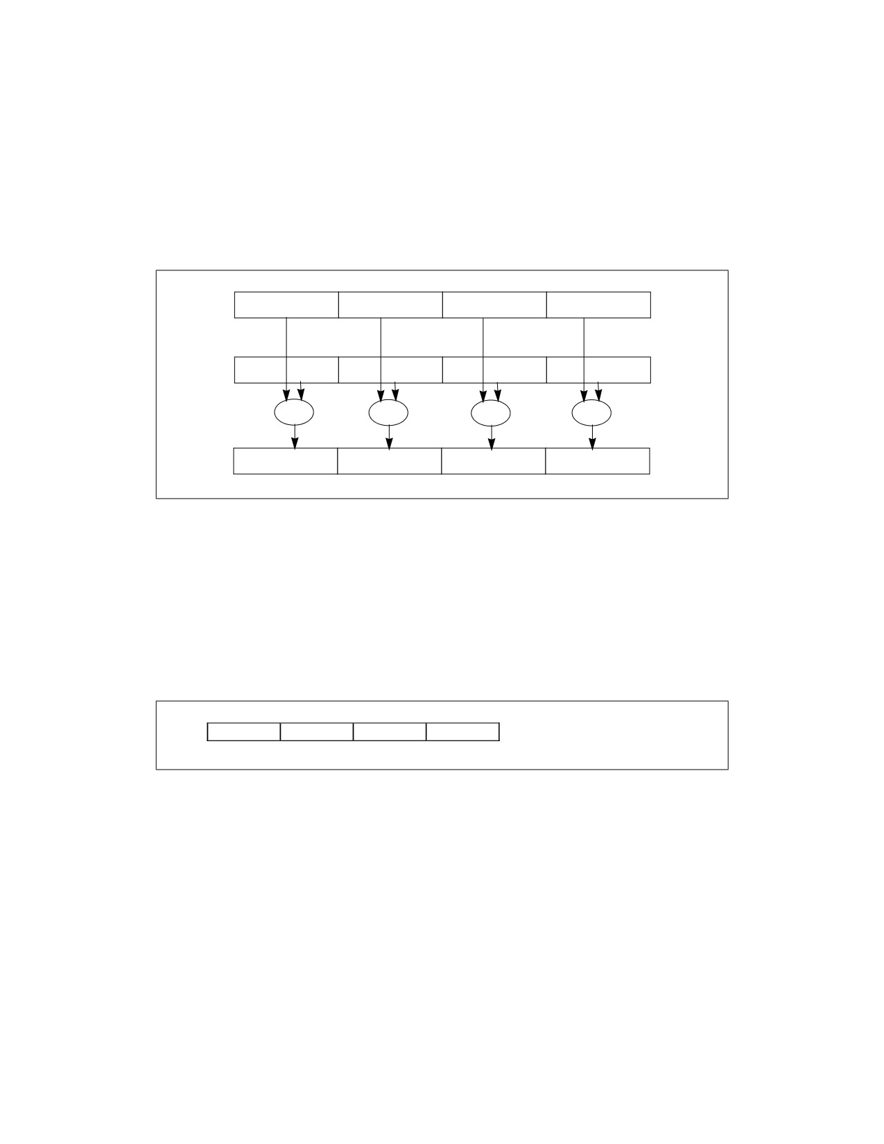
Most floating-point arithmetic instructions in SSE/SSE2 provide a more significant performance gain on
vertical data processing for parallel data elements. This means that each element of the destination
results from an arithmetic operation performed from the source elements in the same vertical position
(Figure 7-1).
To supplement these homogeneous arithmetic operations on parallel data elements, SSE and SSE2
provide data movement instructions (e.g., SHUFPS, UNPCKLPS, UNPCKHPS, MOVLHPS, MOVHLPS, etc.)
that facilitate moving data elements horizontally.
X3
X2
X1
X0
Y3
Y2
Y1
Y0
OP
OP
OP
OP
X3 OP Y3
X2 OP Y2
X 1OP Y1
X0 OP Y0
Figure 7-1. Homogeneous Operation on Parallel Data Elements
The organization of structured data significantly impacts SIMD programming efficiency and performance.
This can be illustrated using two common type of data structure organizations:
• Array of Structure (AoS): This refers to arranging an array of data structures. Within the data
structure, each member is a scalar. This is shown in Figure 7-2. Typically, a repetitive computation
sequence is applied to each element of an array, i.e., a data structure. The computational sequence
for the scalar members of the structure is likely to be non-homogeneous within each iteration. AoS is
generally associated with a horizontal computation model.
X
Y
Z
W
Figure 7-2. Horizontal Computation Model
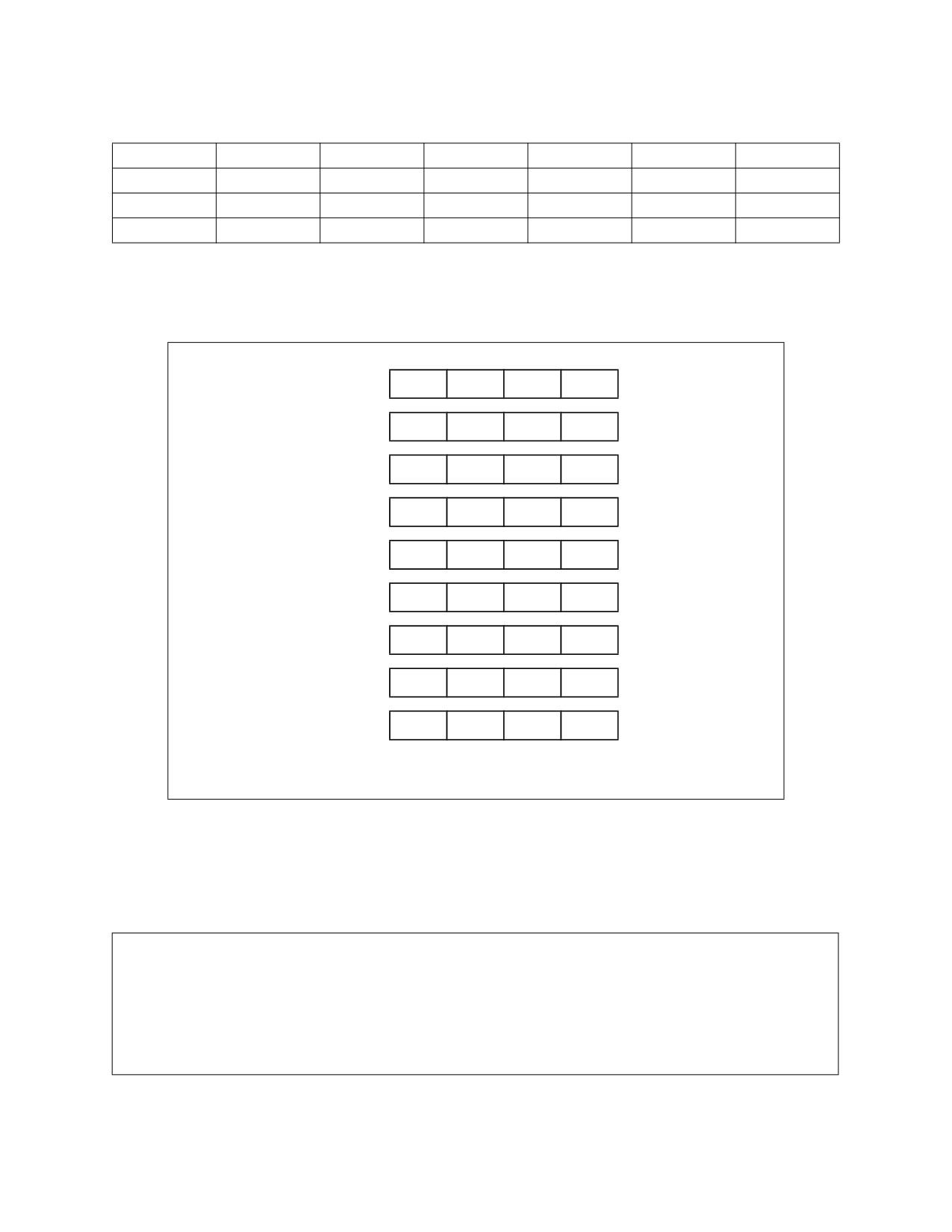
• Structure of Array (SoA): Here, each member of the data structure is an array. Each element of the
array is a scalar. This is shown in Table 7-1. The repetitive computational sequence is applied to
scalar elements and homogeneous operation can be easily achieved across consecutive iterations
within the same structural member. Consequently, SoA is generally amenable to the vertical
computation model.
7-3
OPTIMIZING FOR SIMD FLOATING-POINT APPLICATIONS
Table 7-1. SoA Form of Representing Vertices Data
Vx array
X1
X2
X3
X4
Xn
Vy array
Y1
Y2
Y3
Y4
Yn
Vz array
Z1
Z2
Z3
Y4
Zn
Vw array
W1
W2
W3
W4
Wn
SIMD instructions with vertical computation on the SoA arrangement can achieve higher efficiency and
performance than AoS and horizontal computation. This can be seen with dot-product operation on
vectors. The dot product operation on the SoA arrangement is shown in Figure 7-3.
X1
X2
X3
X4
X
Fx
Fx
Fx
Fx
+
Y1
Y2
Y3
Y4
X
Fy
Fy
Fy
Fy
+
Z1
Z2
Z3
Z4
X
Fz
Fz
Fz
Fz
+
W1
W2
W3
W4
X
Fw
Fw
Fw
Fw
=
R1
R2
R3
R4
OM15168
Figure 7-3. Dot Product Operation
Example 7-1 shows how one result would be computed for seven instructions if the data were organized
as AoS and using SSE alone: four results would require 28 instructions.
Example 7-1. Pseudocode for Horizontal (xyz, AoS) Computation
mulps
; x*x', y*y', z*z'
movaps
; reg->reg move, since next steps overwrite
shufps
; get b,a,d,c from a,b,c,d
addps
; get a+b,a+b,c+d,c+d
movaps
; reg->reg move
shufps
; get c+d,c+d,a+b,a+b from prior addps
addps
; get a+b+c+d,a+b+c+d,a+b+c+d,a+b+c+d
7-4

OPTIMIZING FOR SIMD FLOATING-POINT APPLICATIONS
Now consider the case when the data is organized as SoA. Example 7-2 demonstrates how four results
are computed for five instructions.
Example 7-2. Pseudocode for Vertical (xxxx, yyyy, zzzz, SoA) Computation
mulps
; x*x' for all 4 x-components of 4 vertices
mulps
; y*y' for all 4 y-components of 4 vertices
mulps
; z*z' for all 4 z-components of 4 vertices
addps
; x*x' + y*y'
addps
; x*x'+y*y'+z*z'
For the most efficient use of the four component-wide registers, reorganizing the data into the SoA
format yields increased throughput and hence much better performance for the instructions used.
This simple example shows that vertical computation can yield 100% use of the available SIMD registers
to produce four results. Note that results may vary for other situations. Suppose the data structures are
represented in a format that is not “friendly” to vertical computation. In that case, it can be rearranged
“on the fly” to facilitate better utilization of the SIMD registers. This operation is referred to as a “swiz-
zling” operation. The reverse operation is referred to as “deswizzling.”
7.5.1.2
Data Swizzling
Swizzling data from SoA to AoS format can apply to multiple application domains, including 3D geometry,
video and imaging. Two different swizzling techniques can be adapted to handle floating-point and
integer data. Example 7-3 illustrates a swizzle function that uses SHUFPS, MOVLHPS, and MOVHLPS
instructions.
Example 7-3. Swizzling Data Using SHUFPS, MOVLHPS, MOVHLPS
typedef struct _VERTEX_AOS {
float x, y, z, color;
} Vertex_aos;
// AoS structure declaration
typedef struct _VERTEX_SOA {
float x[4], float y[4], float z[4];
float color[4];
} Vertex_soa;
// SoA structure declaration
void swizzle_asm (Vertex_aos *in, Vertex_soa *out)
{
// in mem: x1y1z1w1-x2y2z2w2-x3y3z3w3-x4y4z4w4-
// SWIZZLE XYZW --> XXXX
asm {
mov rbx, in
// get structure addresses
mov rdx, out
movaps xmm1, [rbx ]
// w0 z0 y0 x0
movaps xmm2, [rbx + 16]
// w1 z1 y1 x1
movaps xmm3, [rbx + 32]
// w2 z2 y2 x2
movaps xmm4, [rbx + 48]
// w3 z3 y2 x3
movaps xmm7, xmm4
// xmm7= w3 z3 y3 x3
movhlps xmm7, xmm3
// xmm7= w3 z3 w2 z2
movaps xmm6, xmm2
// xmm6= w1 z1 y1 x1
movlhps xmm3, xmm4
// xmm3= y3 x3 y1 x1
movhlps xmm2, xmm1
// xmm2= w1 z1 w0 z0
movlhps xmm1, xmm6
// xmm1= y1 x1 y0 x0
7-5

OPTIMIZING FOR SIMD FLOATING-POINT APPLICATIONS
Example 7-3. Swizzling Data (Contd.)Using SHUFPS, MOVLHPS, MOVHLPS (Contd.)
movaps xmm6, xmm2
// xmm6= w1 z1 w0 z0
movaps xmm5, xmm1
// xmm5= y1 x1 y0 x0
shufps xmm2, xmm7, 0xDDh
// xmm2= w3 w2 w1 w0 => W
shufps xmm1, xmm3, 0x88h
// xmm1= x3 x2 x1 x0 => X
shufps xmm5, xmm3, 0xDDh
// xmm5= y3 y2 y1 y0 => Y
shufps xmm6, xmm7, 0x88h
// xmm6= z3 z2 z1 z0 => Z
movaps
[rdx], xmm1
// store X
movaps
[rdx+16], xmm5
// store Y
movaps
[rdx+32], xmm6
// store Z
movaps
[rdx+48], xmm2
// store W
}
}
Example 7-4 shows a similar data-swizzling algorithm using SIMD instructions in the integer domain.
Example 7-4. Swizzling Data Using UNPCKxxx Instructions
void swizzle_asm (Vertex_aos *in, Vertex_soa *out)
{
// in mem: x1y1z1w1-x2y2z2w2-x3y3z3w3-x4y4z4w4-
// SWIZZLE XYZW --> XXXX
asm {
mov rbx, in
// get structure addresses
mov rdx, out
movdqa
xmm1, [rbx + 0*16]
//w0 z0 y0 x0
movdqa
xmm2, [rbx + 1*16]
//w1 z1 y1 x1
movdqa
xmm3, [rbx + 2*16]
//w2 z2 y2 x2
movdqa
xmm4, [rbx + 3*16]
//w3 z3 y3 x3
movdqa
xmm5, xmm1
punpckldq
xmm1, xmm2
// y1 y0 x1 x0
punpckhdq
xmm5, xmm2
// w1 w0 z1 z0
movdqa
xmm2, xmm3
punpckldq
xmm3, xmm4
// y3 y2 x3 x2
punpckhdq
xmm2, xmm4
// w3 w2 z3 z2
movdqa
xmm4, xmm1
punpcklqdq
xmm1, xmm3
// x3 x2 x1 x0
punpckhqdq
xmm4, xmm3
// y3 y2 y1 y0
movdqa
xmm3, xmm5
punpcklqdq
xmm5, xmm2
// z3 z2 z1 z0
punpckhqdq
xmm3, xmm2
// w3 w2 w1 w0
movdqa
[rdx+0*16], xmm1
//x3 x2 x1 x0
movdqa
[rdx+1*16], xmm4
//y3 y2 y1 y0
movdqa
[rdx+2*16], xmm5
//z3 z2 z1 z0
movdqa
[rdx+3*16], xmm3
//w3 w2 w1 w0
}
The technique in Example 7-3 (loading 16 bytes, using SHUFPS and copying halves of XMM registers) is
preferable over an alternate approach of loading halves of each vector using MOVLPS/MOVHPS on newer
microarchitectures. This is because loading 8 bytes using MOVLPS/MOVHPS can create code dependency
and reduce the throughput of the execution engine.
The performance considerations of Example 7-3, and Example 7-4 often depend on each microarchitec-
ture’s characteristics. For example, in Intel Core microarchitecture, executing a SHUFPS tend to be
7-6

OPTIMIZING FOR SIMD FLOATING-POINT APPLICATIONS
slower than a PUNPCKxxx instruction. In Enhanced Intel Core microarchitecture, SHUFPS and PUNP-
CKxxx instruction execute with one cycle throughput due to the 128-bit shuffle execution unit. The next
important consideration is that only one port can execute PUNPCKxxx rather than MOVLHPS/MOVHLPS
executing on multiple ports. The performance of both techniques improves on Intel Core microarchitec-
ture over previous microarchitectures due to 3 ports for executing SIMD instructions. Both techniques
further improve the Enhanced Intel Core microarchitecture due to the 128-bit shuffle unit.
7.5.1.3
Data Deswizzling
In the deswizzle operation, we want to arrange the SoA format back into AoS format so the XXXX, YYYY,
and ZZZZ are rearranged and stored in memory as XYZ. Example 7-5 illustrates one deswizzle function
for floating-point data.
Example 7-5. Deswizzling Single-Precision SIMD Data
void deswizzle_asm(Vertex_soa *in, Vertex_aos *out)
{
__asm {
mov
rcx, in
// load structure addresses
mov
rdx, out
movaps
xmm0, [rcx]
//x3 x2 x1 x0
movaps
xmm1, [rcx + 16]
//y3 y2 y1 y0
movaps
xmm2, [rcx + 32]
//z3 z2 z1 z0
movaps
xmm3, [rcx + 48]
//w3 w2 w1 w0
movaps
xmm5, xmm0
movaps
xmm7, xmm2
unpcklps
xmm0, xmm1
// y1 x1 y0 x0
unpcklps
xmm2, xmm3
// w1 z1 w0 z0
movdqa
xmm4, xmm0
movlhps
xmm0, xmm2
// w0 z0 y0 x0
movhlps
xmm2, xmm4
// w1 z1 y1 x1
unpckhps
xmm5, xmm1
// y3 x3 y2 x2
unpckhps
xmm7, xmm3
// w3 z3 w2 z2
movdqa
xmm6, xmm5
movlhps
xmm5, xmm7
// w2 z2 y2 x2
movhlps
xmm7, xmm6
// w3 z3 y3 x3
movaps
[rdx+0*16], xmm0
//w0 z0 y0 x0
movaps
[rdx+1*16], xmm2
//w1 z1 y1 x1
movaps
[rdx+2*16], xmm5
//w2 z2 y2 x2
movaps
[rdx+3*16], xmm7
//w3 z3 y3 x3
}
}
Example 7-6 shows a similar deswizzle function using SIMD integer instructions. Both techniques
demonstrate loading 16 bytes and performing horizontal data movement in registers. This approach is
likely more efficient than alternative techniques of storing 8-byte halves of XMM registers using MOVLPS
and MOVHPS.
7-7

OPTIMIZING FOR SIMD FLOATING-POINT APPLICATIONS
Example 7-6. Deswizzling Data Using SIMD Integer Instructions
void deswizzle_rgb(Vertex_soa *in, Vertex_aos *out)
{
//---deswizzling---rgb---
// assume: xmm0=rrrr, xmm1=gggg, xmm2=bbbb, xmm3=aaaa
mov
rcx, in
// load structure addresses
mov
rdx, out
movdqa
xmm0, [rcx]
// load r4 r3 r2 r1 => xmm0
movdqa
xmm1, [rcx+16]
// load g4 g3 g2 g1 => xmm1
movdqa
xmm2, [rcx+32]
// load b4 b3 b2 b1 => xmm2
movdqa
xmm3, [rcx+48]
// load a4 a3 a2 a1 => xmm3
// Start deswizzling here
movdqa
xmm5, xmm0
movdqa
xmm7, xmm2
punpckldq
xmm0, xmm1
//g2 r2 g1 r1
punpckldq
xmm2, xmm3
//a2 b2 a1 b1
movdqa
xmm4, xmm0
punpcklqdq
xmm0, xmm2
// a1 b1 g1 r1 => v1
punpckhqdq
xmm4, xmm2
// a2 b2 g2 r2 => v2
punpckhdq
xmm5, xmm1
// g4 r4 g3 r3
punpckhdq
xmm7, xmm3
// a4 b4 a3 b3
movdqa
xmm6, xmm5
punpcklqdq
xmm5, xmm7
// a3 b3 g3 r3 => v3
punpckhqdq
xmm6, xmm7
// a4 b4 g4 r4 => v4
movdqa
[rdx], xmm0
// v1
movdqa
[rdx+16], xmm4
// v2
movdqa
[rdx+32], xmm5
// v3
movdqa
[rdx+48], xmm6
// v4
// DESWIZZLING ENDS HERE
}
}
7.5.1.4
Horizontal ADD Using SSE
Although vertical computations generally use SIMD performance better than horizontal computations,
code must use a horizontal operation in some cases.
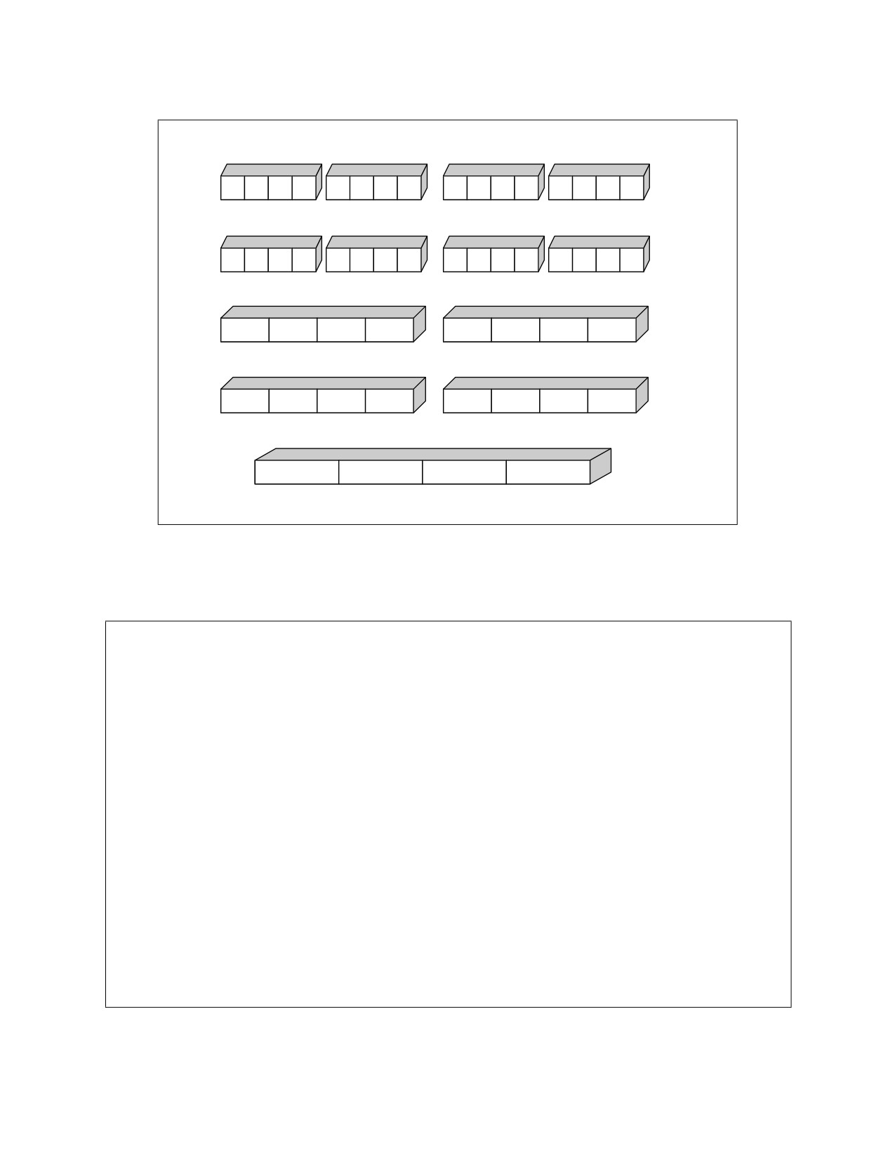
MOVLHPS/MOVHLPS and shuffle can be used to sum data horizontally. For example, starting with four
128-bit registers, to sum up each register horizontally while having the final results in one register, use
the MOVLHPS/MOVHLPS to align the upper and lower parts of each register. This allows you to use a
vertical add. With the resulting partial horizontal summation, full summation follows easily.
Figure 7-4 presents a horizontal add using MOVHLPS/MOVLHPS. Example 7-7 and Example 7-8 provide
the code for this operation.
7-8
OPTIMIZING FOR SIMD FLOATING-POINT APPLICATIONS
xmm0
xmm1
xmm2
xmm3
A1
A2
A3
A4
B1
B2
B3
B4
C1
C2
C3
C4
D1
D2
D3
D4
MOVLHPS
MOVHLPS
MOVLHPS
MOVHLPS
A1
A2
B1
B2
A3
A4
B3
B4
C1
C2
D1
D2
C3
C4
D3
D4
ADDPS
ADDPS
A1+A3
A2+A4
B1+B3
B2+B4
C1+C3
C2+C4
D1+D3
D2+D4
SHUFPS
SHUFPS
A1+A3
B1+B3
C1+C3
D1+D3
A2+A4
B2+B4
C2+C4
D2+D4
ADDPS
A1+A2+A3+A4
B1+B2+B3+B4
C1+C2+C3+C4
D1+D2+D3+D4
OM15169
Figure 7-4. Horizontal Add Using MOVHLPS/MOVLHPS
Example 7-7. Horizontal Add Using MOVHLPS/MOVLHPS
void horiz_add(Vertex_soa *in, float *out) {
__asm {
mov
rcx, in
// load structure addresses
mov
rdx, out
movaps
xmm0, [rcx]
// load A1 A2 A3 A4 => xmm0
movaps
xmm1, [rcx+16]
// load B1 B2 B3 B4 => xmm1
movaps
xmm2, [rcx+32]
// load C1 C2 C3 C4 => xmm2
movaps
xmm3, [rcx+48]
// load D1 D2 D3 D4 => xmm3
// START HORIZONTAL ADD
movaps
xmm5, xmm0
// xmm5= A1,A2,A3,A4
movlhps
xmm5, xmm1
// xmm5= A1,A2,B1,B2
movhlps
xmm1, xmm0
// xmm1= A3,A4,B3,B4
addps
xmm5, xmm1
// xmm5= A1+A3,A2+A4,B1+B3,B2+B4
movaps
xmm4, xmm2
movlhps
xmm2, xmm3
// xmm2= C1,C2,D1,D2
movhlps
xmm3, xmm4
// xmm3= C3,C4,D3,D4
addps
xmm3, xmm2
// xmm3= C1+C3,C2+C4,D1+D3,D2+D4
movaps
xmm6, xmm3
// xmm6= C1+C3,C2+C4,D1+D3,D2+D4
shufps
xmm3, xmm5, 0xDD
//xmm6=A1+A3,B1+B3,C1+C3,D1+D3
shufps
xmm5, xmm6, 0x88
// xmm5= A2+A4,B2+B4,C2+C4,D2+D4
addps
xmm6, xmm5
// xmm6= D,C,B,A
7-9

OPTIMIZING FOR SIMD FLOATING-POINT APPLICATIONS
Example 7-7. Horizontal Add Using MOVHLPS/MOVLHPS (Contd.)
// END HORIZONTAL ADD
movaps
[rdx], xmm6
}
}
Example 7-8. Horizontal Add Using Intrinsics with MOVHLPS/MOVLHPS
void horiz_add_intrin(Vertex_soa *in, float *out)
{
__m128 v, v2, v3, v4;
__m128 tmm0,tmm1,tmm2,tmm3,tmm4,tmm5,tmm6;
// Temporary variables
tmm0 = _mm_load_ps(in->x);
// tmm0 = A1 A2 A3 A4
tmm1 = _mm_load_ps(in->y);
// tmm1 = B1 B2 B3 B4
tmm2 = _mm_load_ps(in->z);
// tmm2 = C1 C2 C3 C4
tmm3 = _mm_load_ps(in->w);
// tmm3 = D1 D2 D3 D4
tmm5 = tmm0;
// tmm0 = A1 A2 A3 A4
tmm5 = _mm_movelh_ps(tmm5, tmm1);
// tmm5 = A1 A2 B1 B2
tmm1 = _mm_movehl_ps(tmm1, tmm0);
// tmm1 = A3 A4 B3 B4
tmm5 = _mm_add_ps(tmm5, tmm1);
// tmm5 = A1+A3 A2+A4 B1+B3 B2+B4
tmm4 = tmm2;
tmm2 = _mm_movelh_ps(tmm2, tmm3);
// tmm2 = C1 C2 D1 D2
tmm3 = _mm_movehl_ps(tmm3, tmm4);
// tmm3 = C3 C4 D3 D4
tmm3 = _mm_add_ps(tmm3, tmm2);
// tmm3 = C1+C3 C2+C4 D1+D3 D2+D4
tmm6 = tmm3;
// tmm6 = C1+C3 C2+C4 D1+D3 D2+D4
tmm6 = _mm_shuffle_ps(tmm3, tmm5, 0xDD);
// tmm6 = A1+A3 B1+B3 C1+C3 D1+D3
tmm5 = _mm_shuffle_ps(tmm5, tmm6, 0x88);
// tmm5 = A2+A4 B2+B4 C2+C4 D2+D4
tmm6 = _mm_add_ps(tmm6, tmm5);
// tmm6 = A1+A2+A3+A4 B1+B2+B3+B4
// C1+C2+C3+C4 D1+D2+D3+D4
_mm_store_ps(out, tmm6);
}
7.5.2
Use of CVTTPS2PI/CVTTSS2SI Instructions
The CVTTPS2PI and CVTTSS2SI instructions implicitly encode the truncate/chop rounding mode in the
instruction. They take precedence over the rounding mode specified in the MXCSR register. This behavior
can eliminate the need to change the rounding mode from round-nearest, to truncate/chop, then return
to round-nearest to resume computation.
Avoid frequent changes to the MXCSR register since a penalty associated with writing this register. Typi-
cally, when using CVTTPS2P/CVTTSS2SI, rounding control in MXCSR can always be set to round-nearest.
7.5.3
Flush-to-Zero and Denormals-are-Zero Modes
The flush-to-zero (FTZ) and denormals-are-zero (DAZ) modes are incompatible with IEEE Standard
7541. They are provided to improve performance for applications where underflow is common and gener-
ating a denormalized result is unnecessary.
1. "IEEE Standard for Floating-Point Arithmetic," in IEEE Std 754-2019 (Revision of IEEE 754-2008) , vol., no., pp.1-84, 22
July 2019, doi: 10.1109/IEEESTD.2019.8766229. https://ieeexplore.ieee.org/document/8766229
7-10
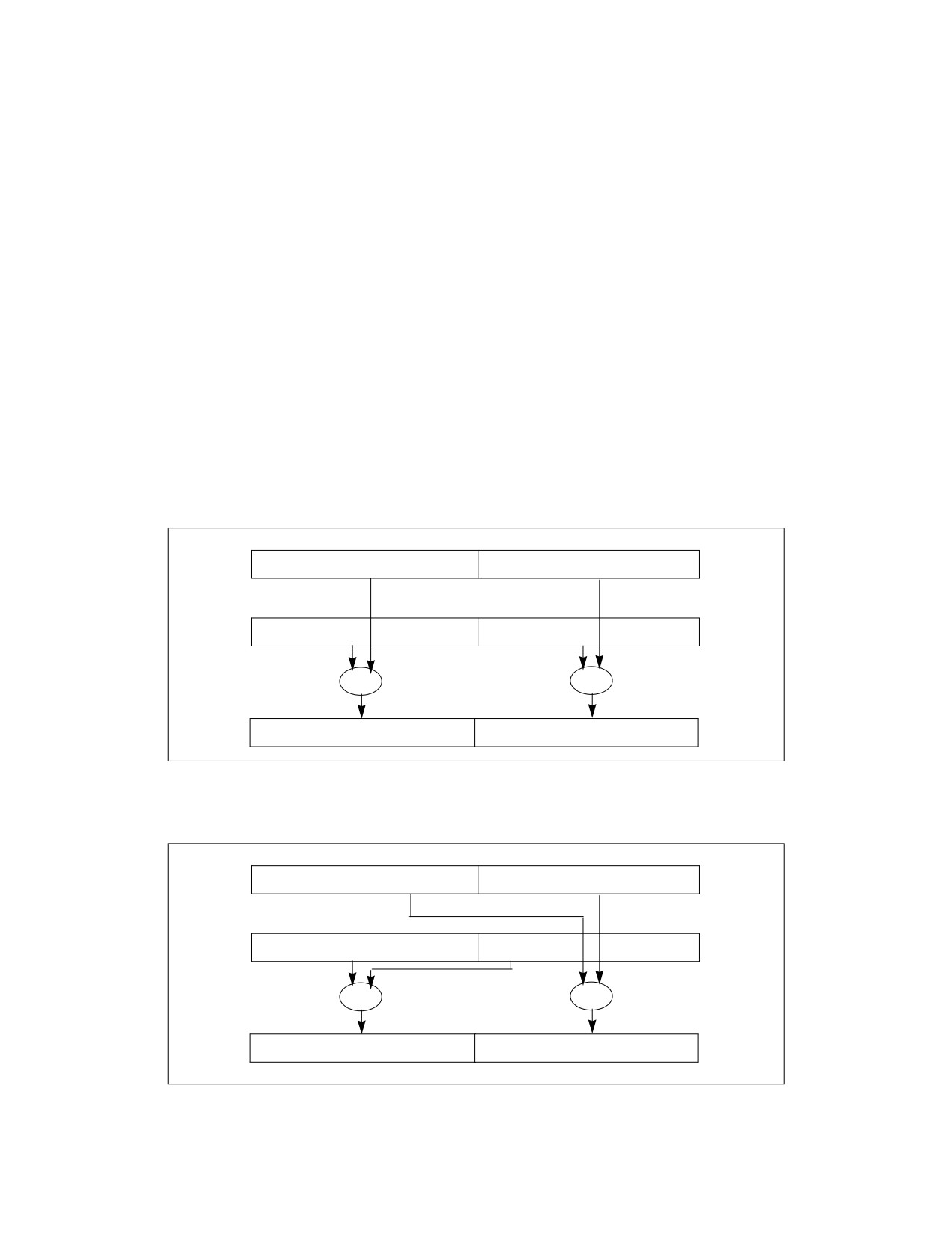
OPTIMIZING FOR SIMD FLOATING-POINT APPLICATIONS
See Section 3.9.2, “Floating-Point Modes and Exceptions.”
7.6
SIMD OPTIMIZATIONS AND MICROARCHITECTURES
Pentium M, Intel Core Solo, and Intel Core Duo processors have a different microarchitecture than the
Intel NetBurst microarchitecture. Intel Core microarchitecture offers significantly more efficient SIMD
floating-point capability than previous microarchitectures. In addition, instruction latency and
throughput of SSE3 instructions are improved considerably in Intel Core microarchitectures over
previous microarchitectures.
7.6.1
SIMD Floating-point Programming Using SSE3
SSE3 enhances SSE and SSE2 with nine instructions targeted for SIMD floating-point programming. In
contrast to many SSE/SSE2 instructions offering homogeneous arithmetic operations on parallel data
elements and favoring the vertical computation model, SSE3 offers instructions that perform asymmetric
arithmetic and arithmetic operations on horizontal data elements.
ADDSUBPS and ADDSUBPD are two instructions with asymmetric arithmetic processing capability (see
Figure 7-5). HADDPS, HADDPD, HSUBPS, and HSUBPD offer horizontal arithmetic processing capability
(see Figure 7-6). In addition: MOVSLDUP, MOVSHDUP, and MOVDDUP load data from memory (or XMM
register) and replicate data elements simultaneously.
X1
X0
Y1
Y0
ADD
SUB
X1 + Y1
X0 -Y0
Figure 7-5. Asymmetric Arithmetic Operation of the SSE3 Instruction
X1
X0
Y1
Y0
ADD
ADD
Y0 + Y1
X0 + X1
Figure 7-6. Horizontal Arithmetic Operation of the SSE3 Instruction HADDPD
7-11

OPTIMIZING FOR SIMD FLOATING-POINT APPLICATIONS
7.6.1.1
SSE3 and Complex Arithmetics
The flexibility of SSE3 in dealing with AOS-type data structures can be demonstrated by the example of
multiplication and division of complex numbers. For example, a complex number can be stored in a struc-
ture consisting of its real and imaginary parts. This naturally leads to the use of an array of structure.
Example 7-9 demonstrates using SSE3 instructions to multiply single-precision complex numbers.
Example 7-10 shows using SSE3 instructions to divide complex numbers.
Example 7-9. Multiplication of Two Pairs of Single-Precision Complex Number
// Multiplication of
(ak + i bk ) * (ck + i dk )
// a + i b can be stored as a data structure
movsldup xmm0, Src1; load real parts into the destination,
; a1, a1, a0, a0
movaps
xmm1, src2; load the 2nd pair of complex values,
; i.e. d1, c1, d0, c0
mulps
xmm0, xmm1; temporary results, a1d1, a1c1, a0d0,
; a0c0
shufps
xmm1, xmm1, b1; reorder the real and imaginary
; parts, c1, d1, c0, d0
movshdup xmm2, Src1; load the imaginary parts into the
; destination, b1, b1, b0, b0
mulps
xmm2, xmm1; temporary results, b1c1, b1d1, b0c0,
; b0d0
addsubps xmm0, xmm2; b1c1+a1d1, a1c1 -b1d1, b0c0+a0d0,
; a0c0-b0d0
Example 7-10. Division of Two Pairs of Single-Precision Complex Numbers
// Division of (ak + i bk ) / (ck + i dk )
movshdup xmm0, Src1; load imaginary parts into the
; destination, b1, b1, b0, b0
movaps
xmm1, src2; load the 2nd pair of complex values,
; i.e. d1, c1, d0, c0
mulps
xmm0, xmm1; temporary results, b1d1, b1c1, b0d0,
; b0c0
shufps
xmm1, xmm1, b1; reorder the real and imaginary
; parts, c1, d1, c0, d0
movsldup xmm2, Src1; load the real parts into the
; destination, a1, a1, a0, a0
mulps
xmm2, xmm1; temp results, a1c1, a1d1, a0c0, a0d0
addsubps
xmm0, xmm2; a1c1+b1d1, b1c1-a1d1, a0c0+b0d0,
; b0c0-a0d0
mulps
xmm1, xmm1; c1c1, d1d1, c0c0, d0d0
movps
xmm2, xmm1;c1c1, d1d1, c0c0, d0d0
shufps
xmm2, xmm2, b1; d1d1, c1c1, d0d0, c0c0
addps
xmm2, xmm1; c1c1+d1d1, c1c1+d1d1, c0c0+d0d0,
; c0c0+d0d0
7-12

OPTIMIZING FOR SIMD FLOATING-POINT APPLICATIONS
Example 7-10. Division of Two Pairs of Single-Precision Complex Numbers (Contd.)
divps xmm0, xmm2
shufps xmm0, xmm0, b1
; (b1c1-a1d1)/(c1c1+d1d1),
; (a1c1+b1d1)/(c1c1+d1d1),
; (b0c0-a0d0)/( c0c0+d0d0),
; (a0c0+b0d0)/( c0c0+d0d0)
In both examples, the complex numbers are stored in arrays of structures. MOVSLDUP, MOVSHDUP, and
the asymmetric ADDSUBPS allow performing complex arithmetic on two pairs of single-precision
complex numbers simultaneously, without unnecessary swizzling between data elements.
Due to microarchitectural differences, software should implement the multiplication of complex double-
precision numbers using SSE3 instructions on processors based on Intel Core microarchitecture. In Intel
Core Duo and Intel Core Solo processors, software should use scalar SSE2 instructions to implement
double-precision complex multiplication. This is because the data path between SIMD execution units is
128 bits in the Intel Core microarchitecture and 64 in previous microarchitectures. Processors based on
the Enhanced Intel Core microarchitecture generally execute SSE3 instruction more efficiently than
previous microarchitectures. They also have a 128-bit shuffle unit that will benefit complex arithmetic
operations further than the Intel Core microarchitecture.
Example 7-11 shows two equivalent implementations of double-precision complex multiplication of two
pairs of complex numbers using vector SSE2 versus SSE3 instructions. Example 7-12 shows the equiva-
lent scalar SSE2 implementation.
Example 7-11. Double-Precision Complex Multiplication of Two Pairs
SSE2 Vector Implementation
SSE3 Vector Implementation
movapd
xmm0, [rax]
;y x
movapd
xmm0, [rax]
;y x
movapd
xmm1, [rax+16]
;w z
movapd
xmm1, [rax+16]
;z z
unpcklpd
xmm1, xmm1
;z z
movapd
xmm2, xmm1
movapd
xmm2, [rax+16]
;w z
unpcklpd
xmm1, xmm1
unpckhpd
xmm2, xmm2
;w w
unpckhpd
xmm2, xmm2
mulpd
xmm1, xmm0
;z*y z*x
mulpd
xmm1, xmm0
;z*y z*x
mulpd
xmm2, xmm0
;w*y w*x
mulpd
xmm2, xmm0
;w*y w*x
xorpd
xmm2, xmm7
;-w*y +w*x
shufpd
xmm2, xmm2, 1
;w*x w*y
shufpd
xmm2, xmm2,1
;w*x -w*y
addsubpd
xmm1, xmm2
;w*x+z*y z*x-w*y
addpd
xmm2, xmm1
;z*y+w*x z*x-w*y
movapd
[rcx], xmm1
movapd
[rcx], xmm2
Example 7-12. Double-Precision Complex Multiplication Using Scalar SSE2
movsd xmm0, [rax]
;x
movsd xmm5, [rax+8]
;y
movsd xmm1, [rax+16]
;z
movsd xmm2, [rax+24]
;w
movsd xmm3, xmm1
;z
movsd xmm4, xmm2
;w
mulsd xmm1, xmm0
;z*x
mulsd xmm2, xmm0
;w*x
mulsd xmm3, xmm5
;z*y
7-13

OPTIMIZING FOR SIMD FLOATING-POINT APPLICATIONS
Example 7-12. Double-Precision Complex Multiplication Using Scalar SSE2 (Contd.)
mulsd xmm4, xmm5
;w*y
subsd xmm1, xmm4
;z*x - w*y
addsd xmm3, xmm2
;z*y + w*x
movsd
[rcx], xmm1
movsd
[rcx+8], xmm3
7.6.1.2
Packed Floating-Point Performance in Intel Core Duo Processor
Most of the packed SIMD floating-point code will speed up on Intel Core Solo processors relative to
Pentium M processors. This is due to an improvement in decoding packed SIMD instructions.
The improved packed floating-point performance on the Intel Core Solo processor over the Pentium M
processor depends on several factors. Generally, decoder-bound code with a mixture of integer and
packed floating-point instructions can expect significant gain. Code that is limited by execution latency
and has a “cycles per instructions” ratio greater than one will not benefit from decoder improvement.
When targeting complex arithmetics on Intel Core Solo and Intel Core Duo processors, single-precision
SSE3 instructions can deliver higher performance than alternatives. On the other hand, tasks requiring
double-precision complex arithmetic may perform better using scalar SSE2 instructions on Intel Core
Solo and Intel Core Duo processors. This is because scalar SSE2 instructions can be dispatched through
two ports and executed using two separate floating-point units.
Packed horizontal SSE3 instructions (HADDPS and HSUBPS) can simplify the code sequence for some
tasks. However, these instructions consist of more than five micro-ops on Intel Core Solo and Intel Core
Duo processors. Care must be taken to ensure the latency and decoding penalty of the horizontal instruc-
tion does not offset any algorithmic benefits.
7.6.2
Dot Product and Horizontal SIMD Instructions
Sometimes the AOS-type of data organization is more natural in many algebraic formulae. One typical
example is the dot product operation. The dot product operation can be implemented using SSE/SSE2
instruction sets. SSE3 added a few horizontal add/subtract instructions for applications that rely on the
horizontal computation model. SSE4.1 provides additional enhancement with instructions capable of
directly evaluating dot product operations of vectors of 2, 3 or 4 components.
Example 7-13. Dot Product of Vector Length 4 Using SSE/SSE2
Using SSE/SSE2 to compute one dot product
movaps
xmm0, [rax]
// a4, a3, a2, a1
mulps
xmm0, [rax+16]
// a4*b4, a3*b3, a2*b2, a1*b1
movhlps
xmm1, xmm0
// X, X, a4*b4, a3*b3, upper half not needed
addps
xmm0, xmm1
// X, X, a2*b2+a4*b4, a1*b1+a3*b3,
pshufd
xmm1, xmm0, 1
// X, X, X, a2*b2+a4*b4
addss
xmm0, xmm1
// a1*b1+a3*b3+a2*b2+a4*b4
movss
[rcx], xmm0
7-14

OPTIMIZING FOR SIMD FLOATING-POINT APPLICATIONS
Example 7-14. Dot Product of Vector Length 4 Using SSE3
Using SSE3 to compute one dot product
movaps
xmm0, [rax]
mulps
xmm0, [rax+16]
// a4*b4, a3*b3, a2*b2, a1*b1
haddps
xmm0, xmm0
// a4*b4+a3*b3, a2*b2+a1*b1, a4*b4+a3*b3, a2*b2+a1*b1
movaps
xmm1, xmm0
// a4*b4+a3*b3, a2*b2+a1*b1, a4*b4+a3*b3, a2*b2+a1*b1
psrlq
xmm0, 32
// 0, a4*b4+a3*b3, 0, a4*b4+a3*b3
addss
xmm0, xmm1
// -, -, -, a1*b1+a3*b3+a2*b2+a4*b4
movss
[rax], xmm0
Example 7-15. Dot Product of Vector Length 4 Using SSE4.1
Using SSE4.1 to compute one dot product
movaps
xmm0, [rax]
dpps
xmm0, [rax+16], 0xf1
// 0, 0, 0, a1*b1+a3*b3+a2*b2+a4*b4
movss
[rax], xmm0
Example 7-13, Example 7-14, and Example 7-15 compare the basic code sequence to compute one dot-
product result for a pair of vectors.
The selection of an optimal sequence in conjunction with an application’s memory access patterns may
favor different approaches. For example, if each dot product result is immediately consumed by addi-
tional computational sequences, it may be more optimal to compare the relative speed of these different
approaches. If dot products can be computed for an array of vectors and kept in the cache for subsequent
computations, then more optimal choice may depend on the relative throughput of the sequence of
instructions.
In Intel Core microarchitecture, Example 7-14 has higher throughput than Example 7-13. Due to the
relatively longer latency of HADDPS, the speed of Example 7-14 is slightly slower than Example 7-13.
In Enhanced Intel Core microarchitecture, Example 7-15 is faster in both speed and throughput than
Example 7-13 and Example 7-14. Although the latency of DPPS is also relatively long, it is compensated
by the reduction of number of instructions in Example 7-15 to do the same amount of work.
Unrolling can further improve the throughput of each of three dot product implementations.
Example 7-16 shows two unrolled versions using the basic SSE2 and SSE3 sequences. The SSE4.1
version can also be unrolled and using INSERTPS to pack 4 dot-product results.
Example 7-16. Unrolled Implementation of Four Dot Products
SSE2 Implementation
SSE3 Implementation
movaps
xmm0, [rax]
movaps
xmm0, [rax]
mulps
xmm0, [rax+16]
;w0*w1 z0*z1 y0*y1 x0*x1
mulps
xmm0, [rax+16]
movaps
xmm2, [rax+32]
movaps
xmm1, [rax+32]
mulps
xmm2, [rax+16+32]
;w2*w3 z2*z3 y2*y3 x2*x3
mulps
xmm1, [rax+16+32]
movaps
xmm3, [rax+64]
movaps
xmm2, [rax+64]
mulps
xmm3, [rax+16+64]
;w4*w5 z4*z5 y4*y5 x4*x5
mulps
xmm2, [rax+16+64]
movaps
xmm4, [rax+96]
movaps
xmm3, [rax+96]
mulps
xmm4, [rax+16+96]
;w6*w7 z6*z7 y6*y7 x6*x7
mulps
xmm3, [rax+16+96]
haddps
xmm0, xmm1
haddps
xmm2, xmm3
haddps
xmm0, xmm2
movaps
[rcx], xmm0
7-15

OPTIMIZING FOR SIMD FLOATING-POINT APPLICATIONS
Example 7-16. Unrolled Implementation of Four Dot Products (Contd.)
SSE2 Implementation
SSE3 Implementation
movaps
xmm1, xmm0
unpcklps
xmm0, xmm2
; y2*y3 y0*y1 x2*x3 x0*x1
unpckhps
xmm1, xmm2
; w2*w3 w0*w1 z2*z3 z0*z1
movaps
xmm5, xmm3
unpcklps
xmm3, xmm4
; y6*y7 y4*y5 x6*x7 x4*x5
unpckhps
xmm5, xmm4
; w6*w7 w4*w5 z6*z7 z4*z5
addps
xmm0, xmm1
addps
xmm5, xmm3
movaps
xmm1, xmm5
movhlps
xmm1, xmm0
movlhps
xmm0, xmm5
addps
xmm0, xmm1
movaps
[rcx], xmm0
7.6.3
Vector Normalization
Normalizing vectors is a common operation in many floating-point applications. Example 7-17 shows an
example in C of normalizing an array of (x, y, z) vectors.
Example 7-17. Normalization of an Array of Vectors
for (i=0;i<CNT;i++)
{ float size = nodes[i].vec.dot();
if (size != 0.0)
{ size = 1.0f/sqrtf(size); }
else
{ size = 0.0; }
nodes[i].vec.x *= size;
nodes[i].vec.y *= size;
nodes[i].vec.z *= size;
}
7-16

OPTIMIZING FOR SIMD FLOATING-POINT APPLICATIONS
Example 7-18 shows an assembly sequence that normalizes the x, y, z components of a vector.
Example 7-18. Normalize (x, y, z) Components of an Array of Vectors Using SSE2
Vec3 *p = &nodes[i].vec;
__asm
{
mov
rax, p
xorps
xmm2, xmm2
movups xmm1, [rax]
// loads the (x, y, z) of input vector plus x of next vector
movaps xmm7, xmm1
// save a copy of data from memory (to restore the unnormalized value)
movaps xmm5, _mask
// mask to select (x, y, z) values from an xmm register to normalize
andps xmm1, xmm5
// mask 1st 3 elements
movaps xmm6, xmm1
// save a copy of (x, y, z) to compute normalized vector later
mulps xmm1,xmm1
// 0, z*z, y*y, x*x
pshufd xmm3, xmm1, 0x1b
// x*x, y*y, z*z, 0
addps xmm1, xmm3
// x*x, z*z+y*y, z*z+y*y, x*x
pshufd xmm3, xmm1, 0x41
// z*z+y*y, x*x, x*x, z*z+y*y
addps xmm1, xmm3
// x*x+y*y+z*z, x*x+y*y+z*z, x*x+y*y+z*z, x*x+y*y+z*z
comisd xmm1, xmm2
// compare size to 0
jz zero
movaps xmm3, xmm4
// preloaded unitary vector (1.0, 1.0, 1.0, 1.0)
sqrtps xmm1, xmm1
divps
xmm3, xmm1
jmp
store
zero:
movaps xmm3, xmm2
store:
mulps xmm3, xmm6
//normalize the vector in the lower 3 elements
andnps xmm5, xmm7
// mask off the lower 3 elements to keep the un-normalized value
orps
xmm3, xmm5
// order the un-normalized component after the normalized vector
movaps
[rax], xmm3
// writes normalized x, y, z; followed by unmodified value
7-17

OPTIMIZING FOR SIMD FLOATING-POINT APPLICATIONS
Example 7-19 shows an assembly sequence using SSE4.1 to normalizes the x, y, z components of a
vector.
Example 7-19. Normalize (x, y, z) Components of an Array of Vectors Using SSE4.1
Vec3 *p = &nodes[i].vec;
__asm
{
mov
rax, p
xorps
xmm2, xmm2
movups xmm1, [rax]
// loads the (x, y, z) of input vector plus x of next vector
movaps xmm7, xmm1
// save a copy of data from memory
dpps
xmm1, xmm1, 0x7f
// x*x+y*y+z*z, x*x+y*y+z*z, x*x+y*y+z*z, x*x+y*y+z*z
comisd
xmm1, xmm2
// compare size to 0
jz zero
movaps xmm3, xmm4
// preloaded unitary vector (1.0, 1.0, 1.0, 1.0)
sqrtps xmm1, xmm1
divps
xmm3, xmm1
jmp
store
zero:
movaps xmm3, xmm2
store:
mulps xmm3, xmm6
//normalize the vector in the lower 3 elements
blendps xmm3, xmm7, 0x8
// copy the un-normalized component next to the normalized vector
movaps
[rax], xmm3
In Example 7-18 and Example 7-19, the throughput of these instruction sequences are basically limited
by the long-latency instructions of DIVPS and SQRTPS. In Example 7-19, the use of DPPS replaces eight
SSE2 instructions to evaluate and broadcast the dot-product result to four elements of an XMM register.
This could result in improvement of the relative speed of Example 7-19 over Example 7-18.
7.6.4
Using Horizontal SIMD Instruction Sets and Data Layout
SSE and SSE2 provide packed add/subtract, multiply/divide instructions that are ideal for situations that
can take advantage of vertical computation model, such as SOA data layout. SSE3 and SSE4.1 added
horizontal SIMD instructions including horizontal add/subtract, dot-product operations. These more
recent SIMD extensions provide tools to solve problems involving data layouts or operations that do not
conform to the vertical SIMD computation model.
In this section, we consider a vector-matrix multiplication problem and discuss the relevant factors for
choosing various horizontal SIMD instructions.
7-18

OPTIMIZING FOR SIMD FLOATING-POINT APPLICATIONS
Example 7-20 shows the vector-matrix data layout in AOS, where the input and out vectors are stored as
an array of structure.
Example 7-20. Data Organization in Memory for AOS Vector-Matrix Multiplication
Matrix M4x4 (pMat):
M00 M01 M02 M03
M10 M11 M12 M13
M20 M21 M22 M23
M30 M31 M32 M33
4 input vertices V4x1 (pVert):
V0x V0y V0z V0w
V1x V1y V1z V1w
V2x V2y V2z V2w
V3x V3y V3z V3w
Output vertices O4x1 (pOutVert): O0x O0y O0z O0w
O1x O1y O1z O1w
O2x O2y O2z O2w
O3x O3y O3z O3w
Example 7-21 shows an example using HADDPS and MULPS to perform vector-matrix multiplication with
data layout in AOS. After three HADDPS completing the summations of each output vector component,
the output components are arranged in AOS.
Example 7-21. AOS Vector-Matrix Multiplication with HADDPS
mov
rax, pMat
mov
rbx, pVert
mov
rcx, pOutVert
xor
rdx, rdx
movaps
xmm5,[rax+16]
// load row M1?
movaps
xmm6,[rax+2*16]
// load row M2?
movaps
xmm7,[rax+3*16]
// load row M3?
lloop:
movaps
xmm4, [rbx + rdx]
// load input vector
movaps
xmm0, xmm4
mulps
xmm0, [rax]
// m03*vw, m02*vz, m01*vy, m00*vx,
movaps
xmm1, xmm4
mulps
xmm1, xmm5
// m13*vw, m12*vz, m11*vy, m10*vx,
movaps
xmm2, xmm4
mulps
xmm2, xmm6
// m23*vw, m22*vz, m21*vy, m20*vx
movaps
xmm3, xmm4
mulps
xmm3, xmm7
// m33*vw, m32*vz, m31*vy, m30*vx,
haddps
xmm0, xmm1
haddps
xmm2, xmm3
haddps
xmm0, xmm2
movaps
[rcx + rdx], xmm0
// store a vector of length 4
add
rdx, 16
cmp
rdx, top
jb lloop
7-19

OPTIMIZING FOR SIMD FLOATING-POINT APPLICATIONS
Example 7-22 shows an example using DPPS to perform vector-matrix multiplication in AOS.
Example 7-22. AOS Vector-Matrix Multiplication with DPPS
mov
rax, pMat
mov
rbx, pVert
mov
rcx, pOutVert
xor
rdx, rdx
movaps xmm5,[rax+16]
// load row M1?
movaps xmm6,[rax+2*16]
// load row M2?
movaps xmm7,[rax+3*16]
// load row M3?
lloop:
movaps xmm4, [rbx + rdx]
// load input vector
movaps xmm0, xmm4
dpps
xmm0, [rax], 0xf1
// calculate dot product of length 4, store to lowest dword
movaps xmm1, xmm4
dpps
xmm1, xmm5, 0xf1
movaps xmm2, xmm4
dpps
xmm2, xmm6, 0xf1
movaps xmm3, xmm4
dpps
xmm3, xmm7, 0xf1
movss
[rcx + rdx + 0*4], xmm0
// store one element of vector length 4
movss
[rcx + rdx + 1*4], xmm1
movss
[rcx + rdx + 2*4], xmm2
movss
[rcx + rdx + 3*4], xmm3
add
rdx, 16
cmp
rdx, top
jb
lloop
Example 7-21 and Example 7-22 both work with AOS data layout using different horizontal processing
techniques provided by SSE3 and SSE4.1. The effectiveness of either techniques will vary, depending on
the degree of exposures of long-latency instruction in the inner loop, the overhead/efficiency of data
movement, and the latency of HADDPS vs. DPPS.
On processors that support both HADDPS and DPPS, the choice between either technique may depend on
application-specific considerations. If the output vectors are written back to memory directly in a batch
situation, Example 7-21 may be preferable over Example 7-22, because the latency of DPPS is long and
storing each output vector component individually is less than ideal for storing an array of vectors.
There may be partially-vectorizable situations that the individual output vector component is consumed
immediately by other non-vectorizable computations. Then, using DPPS producing individual component
may be more suitable than dispersing the packed output vector produced by three HADDPS as in
Example 7-21.
7.6.4.1
SOA and Vector Matrix Multiplication
If the native data layout of a problem conforms to SOA, then vector-matrix multiply can be coded using
MULPS, ADDPS without using the longer-latency horizontal arithmetic instructions, or packing scalar
components into packed format (Example 7-22). To achieve higher throughput with SOA data layout,
there are either prerequisite data preparation or swizzling/deswizzling on-the-fly that must be compre-
hended. For example, an SOA data layout for vector-matrix multiplication is shown in Example 7-23.
7-20

OPTIMIZING FOR SIMD FLOATING-POINT APPLICATIONS
Each matrix element is replicated four times to minimize data movement overhead for producing packed
results.
Example 7-23. Data Organization in Memory for SOA Vector-Matrix Multiplication
Matrix M16x4 (pMat):
M00 M00 M00 M00 M01 M01 M01 M01 M02 M02 M02 M02 M03 M03 M03 M03
M10 M10 M10 M10 M11 M11 M11 M11 M12 M12 M12 M12 M13 M13 M13 M13
M20 M20 M20 M20 M21 M21 M21 M21 M22 M22 M22 M22 M23 M23 M23 M23
M30 M30 M30 M30 M31 M31 M31 M31 M32 M32 M32 M32 M33 M33 M33 M33
4 input vertices V4x1 (pVert): V0x V1x V2x V3x
V0y V1y V2y V3y
V0z V1z V2z V3z
V0w V1w V2w V3w
Ouput vertices O4x1 (pOutVert): O0x O1x O2x O3x
O0y O1y O2y O3y
O0z O1z O2z O3z
O0w O1w O2w O3w
7-21

OPTIMIZING FOR SIMD FLOATING-POINT APPLICATIONS
The corresponding vector-matrix multiply example in SOA (unrolled for four iteration of vectors) is shown
in Example 7-24.
Example 7-24. Vector-Matrix Multiplication with Native SOA Data Layout
mov
rbx, pVert
mov
rcx, pOutVert
xor
rdx, rdx
movaps
xmm5,[rax + 16]
// load row M1?
movaps
xmm6,[rax + 2*16]
// load row M2?
movaps
xmm7,[rax + 3*16]
// load row M3?
lloop_vert:
mov
rax, pMat
xor
edi, edi
movaps
xmm0, [rbx]
// load V3x, V2x, V1x, V0x
movaps
xmm1, [rbx]
// load V3y, V2y, V1y, V0y
movaps
xmm2, [rbx]
// load V3z, V2z, V1z, V0z
movaps
xmm3, [rbx]
// load V3w, V2w, V1w, V0w
loop_mat:
movaps
xmm4, [rax]
// m00, m00, m00, m00,
mulps
xmm4, xmm0
// m00*V3x, m00*V2x, m00*V1x, m00*V0x,
movaps
xmm4, [rax + 16]
// m01, m01, m01, m01,
mulps
xmm5, xmm1
// m01*V3y, m01*V2y, m01*V1y, m01*V0y,
addps
xmm4, xmm5
movaps
xmm5, [rax + 32]
// m02, m02, m02, m02,
mulps
xmm5, xmm2
// m02*V3z, m02*V2z, m02*V1z, m02*V0z,
addps
xmm4, xmm5
movaps
xmm5, [rax+ 48]
// m03, m03, m03, m03,
mulps
xmm5, xmm3
// m03*V3w, m03*V2w, m03*V1w, m03*V0w,
addps
xmm4, xmm5
movaps
[rcx + rdx], xmm4
add
rax, 64
add
rdx, 16
add
edi, 1
cmp
edi, 4
jb lloop_mat
add
rbx, 64
cmp
rdx, top
jb lloop_vert
7-22
7.
Updates to Chapter 10
Change bars and violet text show changes to Chapter 10 of the Intel® 64 and IA-32 Architectures Optimization
Resource Manual: Sub-NUMA Clustering.
------------------------------------------------------------------------------------------
Changes to this chapter:
• Section 10.3:
— Consolidated links and page titles where necessary.
— Removed dead link to Intel blog.
Intel® 64 and IA-32 Architectures Optimization Reference Manual Documentation Changes
13
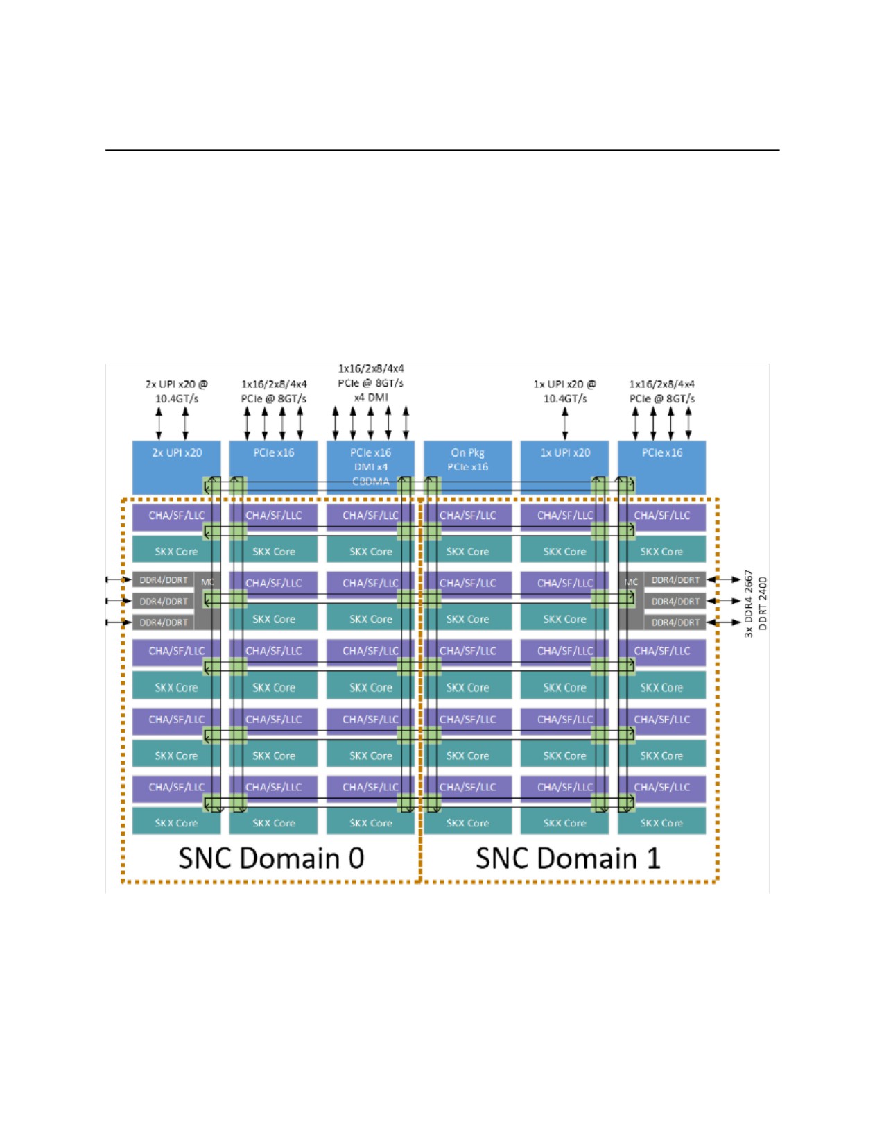
CHAPTER 10
SUB-NUMA CLUSTERING
Sub-NUMA Clustering (SNC) is a mode for improving average latency from last level cache (LLC) to local
memory. It replaces the Cluster-on-Die (COD) implementation which was used in the previous genera-
tion of the Intel® Xeon® processor E5 family.
10.1
SUB-NUMA CLUSTERING
SNC can improve the average LLC/memory latency by splitting the LLC into disjoint clusters based on
address range, with each cluster bound to a subset of memory controllers in the system.
Figure 10-1. Example of SNC Configuration
SUB-NUMA CLUSTERING
10.2
COMPARISON WITH CLUSTER-ON-DIE
SNC provides similar localization benefits to those of COD, but without some of COD’s disadvantages.
Unlike COD, SNC has the following properties.
• Only one Ultra Path Interconnect (UPI) caching agent is required.
• Memory access latency in remote clusters is smaller, as no UPI flow is needed.
• It uses LLC capacity more efficiently as there is no duplication of lines in the LLC.
A disadvantage of SNC is listed below.
• Remote cluster addresses are never cached in local cluster LLC, resulting in larger latency
compared to Cluster-on-Die (COD) in some cases.
10.3
SNC USAGE
This section describes the following modes and their BIOS names in brackets (the exact BIOS parameter
names may vary depending on the BIOS vendor and version).
• NUMA disabled (NUMA Optimized: Disabled)
• SNC off (Integrated Memory Controller (IMC) Interleaving: auto, NUMA Optimized: Enabled,
Sub_NUMA Cluster: Disabled)
• SNC on (IMC Interleaving: 1-way Interleave, NUMA Optimized: Enabled, Sub_NUMA Cluster:
Enabled)
The commands that follow were executed on a 2-socket Intel® Xeon® system, 28 cores per a socket,
Intel® Hyper-Threading Technology enabled.
10.3.1 How to Check NUMA Configuration
There are additional NUMA nodes in a system with SNC enabled; to get benefits from the SNC feature, a
developer should be aware of the NUMA configuration.
This chapter describes different ways to check NUMA system configuration.
libnuma
An application can check NUMA configuration with libnuma.
As an example this code uses the libnuma library to find the maximum number of NUMA nodes.
#include <stdio.h>
#include <stdlib.h>
#include <numa.h>
int main(int argc, char *argv[])
{
int max_node;
/* Check the system for NUMA support */
max_node = numa_max_node();
printf("%d\n", max_node);
10-2
SUB-NUMA CLUSTERING
return 0;
}
numactl
In Linux* you can check the NUMA configuration with the numactl utility (the numactl-libs, and
numactl-devel packages might also be required).
$ numactl --hardware
NUMA disabled:
available: 1 nodes (0)
node 0 cpus: 0 1 2 3 4 5 6 7 8 9 10 11 12 13 14 15 16 17 18 19 20 21 22
23 24 25 26 27 28 29 30 31 32 33 34 35 36 37 38 39 40 41 42 43 44 45 46
47 48 49 50 51 52 53 54 55 56 57 58 59 60 61 62 63 64 65 66 67 68 69 70
71 72 73 74 75 76 77 78 79 80 81 82 83 84 85 86 87 88 89 90 91 92 93 94
95 96 97 98 99 100 101 102 103 104 105 106 107 108 109 110 111
node 0 size: 196045 MB
node 0 free: 190581 MB
node distances:
node
0
0:
10
SNC off:
available: 2 nodes (0-1)
node 0 cpus: 0 1 2 3 4 5 6 7 8 9 10 11 12 13 14 15 16 17 18 19 20 21 22
23 24 25 26 27 56 57 58 59 60 61 62 63 64 65 66 67 68 69 70 71 72 73 74
75 76 77 78 79 80 81 82 83
node 0 size: 96973 MB
node 0 free: 94089 MB
node 1 cpus: 28 29 30 31 32 33 34 35 36 37 38 39 40 41 42 43 44 45 46 47
48 49 50 51 52 53 54 55 84 85 86 87 88 89 90 91 92 93 94 95 96 97 98 99
100 101 102 103 104 105 106 107 108 109 110 111
node 1 size: 98304 MB
node 1 free: 95694 MB
node distances:
node
0
1
0:
10
21
1:
21
10
10-3
SUB-NUMA CLUSTERING
SNC on:
available: 4 nodes (0-3)
node 0 cpus: 0 1 2 3 7 8 9 14 15 16 17 21 22 23 56 57 58 59 63 64 65 70
71 72 73 77 78 79
node 0 size: 47821 MB
node 0 free: 45759 MB
node 1 cpus: 4 5 6 10 11 12 13 18 19 20 24 25 26 27 60 61 62 66 67 68 69
74 75 76 80 81 82 83
node 1 size: 49152 MB
node 1 free: 47097 MB
node 2 cpus: 28 29 30 31 35 36 37 42 43 44 45 49 50 51 84 85 86 87 91 92
93 98 99 100 101 105 106 107
node 2 size: 49152 MB
node 2 free: 47617 MB
node 3 cpus: 32 33 34 38 39 40 41 46 47 48 52 53 54 55 88 89 90 94 95 96
97 102 103 104 108 109 110 111
node 3 size: 49152 MB
node 3 free: 47231 MB
node distances:
node
0
1
2
3
0:
10
11
21
21
1:
11
10
21
21
2:
21
21
10
11
3:
21
21
11
10
hwloc
In Linux* you can also check the NUMA configuration with the lstopo utility (the hwloc package is
required). For example:
$ lstopo -p --of png --no-io --no-caches > numa_topology.png
10-4
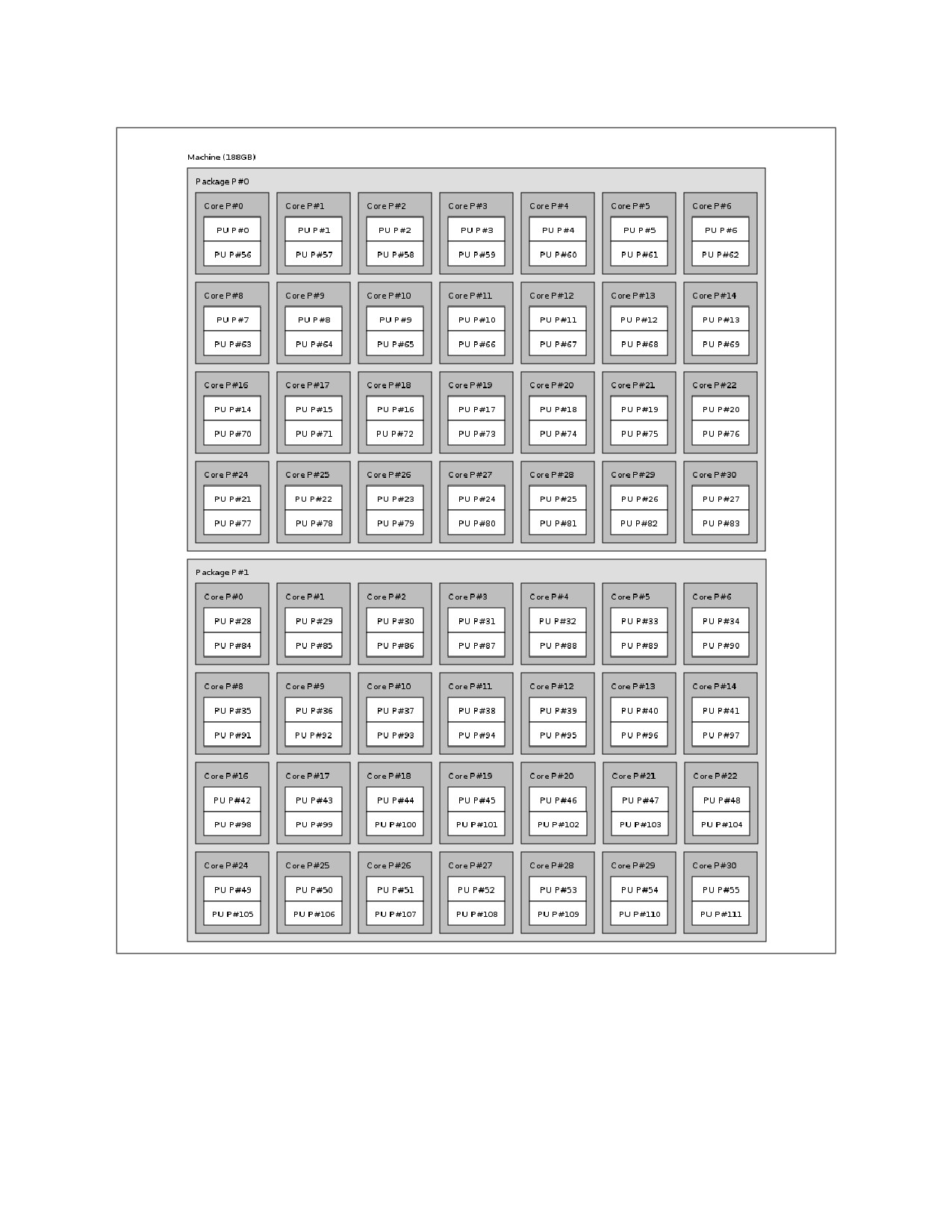
SUB-NUMA CLUSTERING
Figure 10-2. NUMA Disabled
10-5
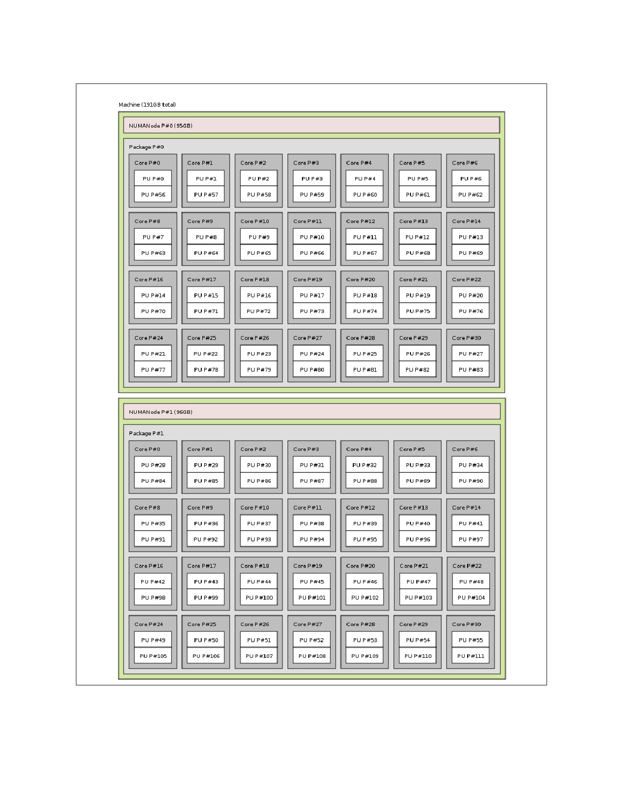
SUB-NUMA CLUSTERING
Figure 10-3. SNC Off
10-6
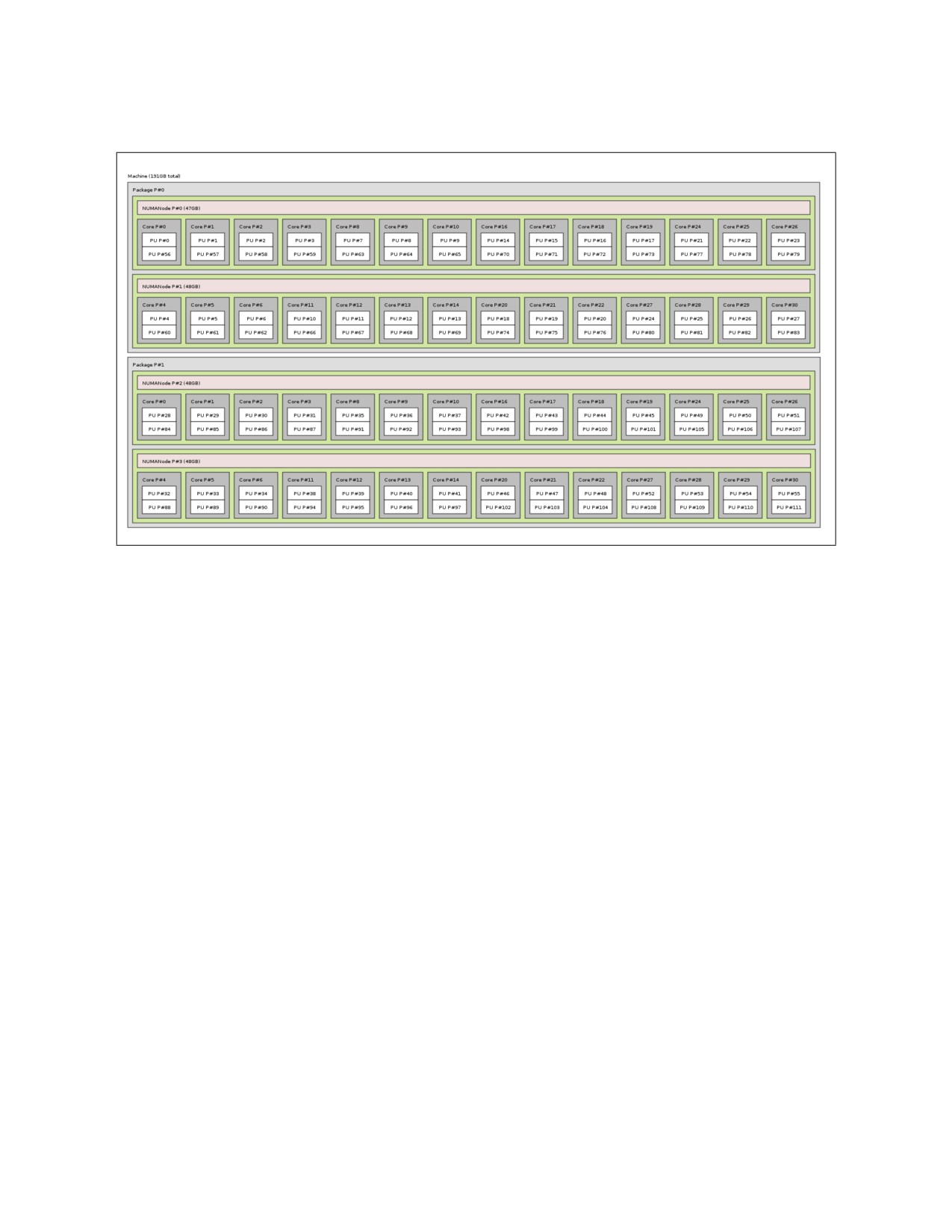
SUB-NUMA CLUSTERING
Figure 10-4. SNC On
10.3.2 MPI Optimizations for SNC
Software needs to be NUMA optimized to benefit from SNC. Running one MPI rank per NUMA region
trivially ensures locality-of-access without requiring changes to the code to ensure that it behaves in a
NUMA friendly manner. This is a simple way to improve performance through the use of SNC.
The Intel® MPI Library includes some NUMA-related optimizations. The out-of-the-box behavior of the
Intel MPI Library should cover most cases, but there are some environment variables available to
control NUMA-related features that can improve performance in specific cases.
The relevant environment variables mainly relate to MPI process placement, that is, process
pinning/binding - such as the I_MPI_PIN_DOMAIN variable. For more information, see the Intel® MPI
Library Developer Reference. This environment variable defines a number of non-overlapping subsets
(domains) of logical processors on a node, and a set of rules for how MPI processes are bound to these
domains: one MPI process per domain, as illustrated below.
10-7
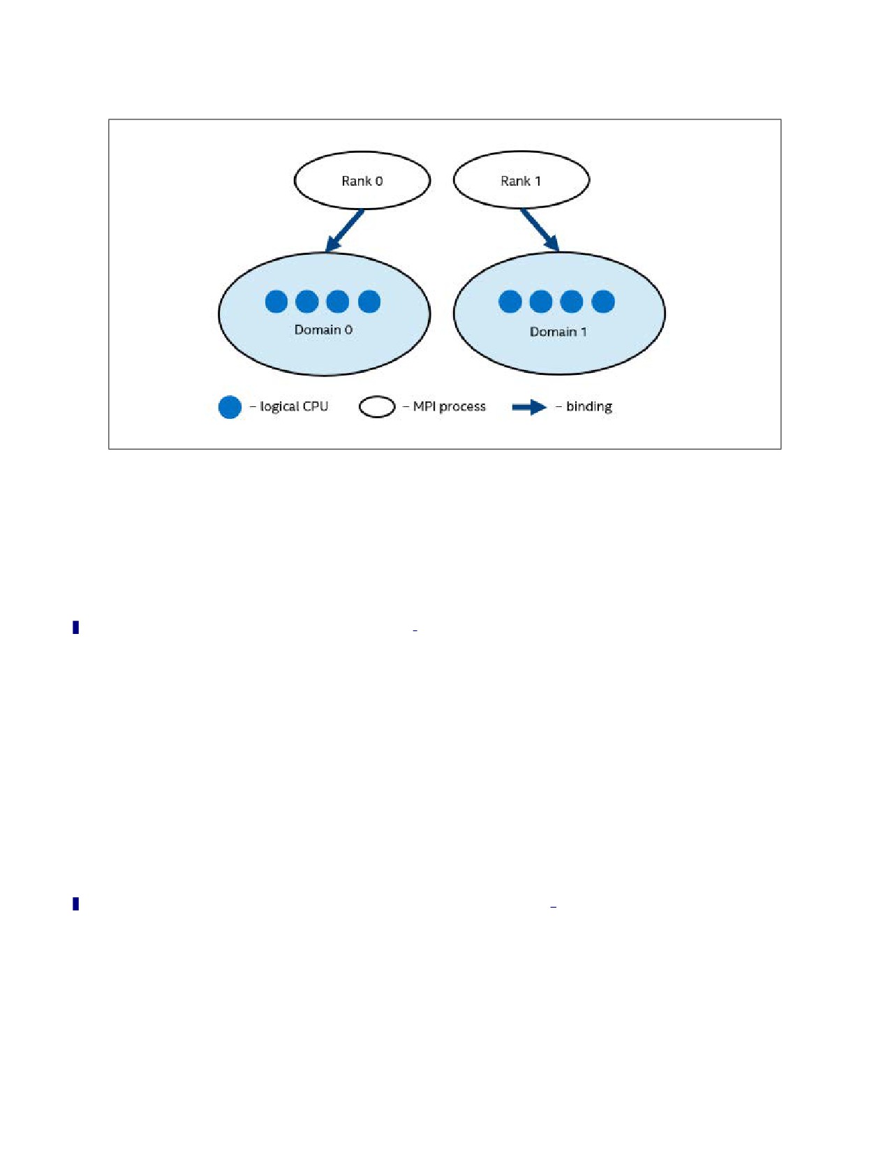
SUB-NUMA CLUSTERING
Figure 10-5. Domain Example with One MPI Process Per Domain
Each MPI process can create a number of child threads to run within the corresponding domain. The
process’ threads can freely migrate from one logical processor to another within the particular domain.
For example, I_MPI_PIN_DOMAIN=numa may be a reasonable option for hybrid MPI/OpenMP* appli-
cations with SNC mode enabled. In this case, each domain consists of logical processors that share a
particular NUMA node. The number of domains on a machine is equal to the number of NUMA nodes on
the machine.
Please see the Intel MPI Library documentation for detailed information.
10.3.3 SNC Performance Comparison
This section contains performance data collected with Intel® Memory Latency Checker (Intel® MLC) to
demonstrate the variations in performance (latency) between NUMA nodes in different modes.
An important factor in determining application performance is the time required for the application to
fetch data from the processor’s cache hierarchy and from the memory subsystem. Local memory and
cross-socket memory latencies vary significantly in a NUMA-enabled multi-socket system. Bandwidth
also plays an important role in determining performance. So measuring these latencies and bandwidths
is important when establishing a baseline for the system being tested, and performing performance anal-
ysis.
Intel MLC is a tool used to measure memory latencies and bandwidth, and how they change as the load
on the system increases. It also provides several options for more fine-grained investigation where band-
width and latencies from a specific set of cores to caches or memory can be measured as well.
For details, see Intel® Memory Latency Checker v.3.10 (Intel® MLC).
The following command was used to collect the performance data:
% mlc_avx512 --latency_matrix
This command measures idle memory latency from each socket in the system to every other socket and
reports the results in a matrix. The default invocation reports latencies to all of the NUMA nodes in the
system. NUMA-level reporting works only on Linux. On Windows, only socket level reporting is supported.
10-8
SUB-NUMA CLUSTERING
NOTE
It is challenging to measure memory latencies on modern Intel processors accurately as
they have sophisticated HW prefetchers. Intel MLC automatically disables these
prefetchers while measuring the latencies and restores them to their previous state on
completion. The prefetcher control is exposed through an MSR and MSR access requires
root level permission. So, Intel MLC needs to be run as ‘root’ on Linux.
The software configuration used for these measurements is Intel MLC v3.3-Beta2, Red Hat* Linux* 7.2.
NUMA disabled:
Using buffer size of 2000.000MB
Measuring idle latencies (in ns)...
Memory node
Socket
0
1
0
126.5
129.4
1
123.1
122.6
SNC off:
Using buffer size of 2000.000MB
Measuring idle latencies (in ns)...
Numa node
Numa node
0
1
0
81.9
153.1
1
153.7
82.0
SNC on:
Using buffer size of 2000.000MB
Measuring idle latencies (in ns)...
Numa node
Numa node
0
1
2
3
0
81.6
89.4
140.4
153.6
1
86.5
78.5
144.3
162.8
2
142.3
153.0
81.6
89.3
3
144.5
162.8
85.5
77.4
10-9
SUB-NUMA CLUSTERING
10-10
6.
Updates to Chapter 11
Change bars and violet text show changes to Chapter 11 of the Intel® 64 and IA-32 Architectures Optimization
Resource Manual: Multicore and Hyper-Threading Technology.
------------------------------------------------------------------------------------------
Changes to this chapter:
• Section 11.4.1: Updated and consolidated outdated link within document title.
• Section 11.4.2: Removed dead link for: Using Spin-Loops on Intel Pentium 4 Processor and Intel Xeon
Processor.
Intel® 64 and IA-32 Architectures Optimization Reference Manual Documentation Changes
13

CHAPTER 11
MULTICORE AND INTEL® HYPER-THREADING TECHNOLOGY (INTEL® HT)
This chapter describes software optimization techniques for multithreaded applications running in an
environment using either multiprocessor (MP) systems or processors with hardware-based multi-
threading support. Multiprocessor systems are systems with two or more sockets, each mated with a
physical processor package. Intel 64 and IA-32 processors that provide hardware multithreading support
include dual-core processors, quad-core processors and processors supporting HT Technology1.
Computational throughput in a multithreading environment can increase as more hardware resources
are added to take advantage of thread-level or task-level parallelism. Hardware resources can be added
in the form of more than one physical-processor, processor-core-per-package, and/or logical-processor-
per-core. Therefore, there are some aspects of multithreading optimization that apply across MP, multi-
core, and HT Technology. There are also some specific microarchitectural resources that may be imple-
mented differently in different hardware multithreading configurations (for example: execution
resources are not shared across different cores but shared by two logical processors in the same core if
HT Technology is enabled). This chapter covers guidelines that apply to these situations.
This chapter covers:
• Performance characteristics and usage models.
• Programming models for multithreaded applications.
• Software optimization techniques in five specific areas.
11.1
PERFORMANCE AND USAGE MODELS
The performance gains of using multiple processors, multicore processors or HT Technology are greatly
affected by the usage model and the amount of parallelism in the control flow of the workload. Two
common usage models are:
• Multithreaded applications.
• Multitasking using single-threaded applications.
11.1.1 Multithreading
When an application employs multithreading to exploit task-level parallelism in a workload, the control
flow of the multi-threaded software can be divided into two parts: parallel tasks and sequential tasks.
Amdahl’s law describes an application’s performance gain as it relates to the degree of parallelism in the
control flow. It is a useful guide for selecting the code modules, functions, or instruction sequences that
are most likely to realize the most gains from transforming sequential tasks and control flows into
parallel code to take advantage multithreading hardware support.
Figure 11-1 illustrates how performance gains can be realized for any workload according to Amdahl’s
law. The bar in Figure 11-1 represents an individual task unit or the collective workload of an entire
application.
1. The presence of hardware multithreading support in Intel 64 and IA-32 processors can be detected by checking the fea-
ture flag CPUID .01H:EDX[28]. A return value of in bit 28 indicates that at least one form of hardware multithreading is
present in the physical processor package. The number of logical processors present in each package can also be
obtained from CPUID. The application must check how many logical processors are enabled and made available to appli-
cation at runtime by making the appropriate operating system calls. See the Intel® 64 and IA-32 Architectures Software
Developer’s Manual, Volume 2A for information.
MULTICORE AND INTEL® HYPER-THREADING TECHNOLOGY (INTEL® HT)
In general, the speed-up of running multiple threads on an MP systems with N physical processors, over
single-threaded execution, can be expressed as:
-
RelativeResponse
= --------------------------------
=
1-P
+ -+O
Tparallel
N
where P is the fraction of workload that can be parallelized, and O represents the overhead of multi-
threading and may vary between different operating systems. In this case, performance gain is the
inverse of the relative response.
Tsequential
Single Thread
1-P
P
Tparallel
P/2
Multi-Thread on MP
1-P
P/2
Figure 11-1. Amdahl’s Law and MP Speed-up
When optimizing application performance in a multithreaded environment, control flow parallelism is
likely to have the largest impact on performance scaling with respect to the number of physical proces-
sors and to the number of logical processors per physical processor.
If the control flow of a multi-threaded application contains a workload in which only 50% can be executed
in parallel, the maximum performance gain using two physical processors is only 33%, compared to using
a single processor. Using four processors can deliver no more than a 60% speed-up over a single
processor. Thus, it is critical to maximize the portion of control flow that can take advantage of parallelism.
Improper implementation of thread synchronization can significantly increase the proportion of serial
control flow and further reduce the application’s performance scaling.
In addition to maximizing the parallelism of control flows, interaction between threads in the form of
thread synchronization and imbalance of task scheduling can also impact overall processor scaling
significantly.
Excessive cache misses are one cause of poor performance scaling. In a multithreaded execution envi-
ronment, they can occur from:
• Aliased stack accesses by different threads in the same process.
• Thread contentions resulting in cache line evictions.
• False-sharing of cache lines between different processors.
Techniques that address each of these situations (and many other areas) are described in sections in this
chapter.
11.1.2 Multitasking Environment
Hardware multithreading capabilities in Intel 64 and IA-32 processors can exploit task-level parallelism
when a workload consists of several single-threaded applications and these applications are scheduled to
run concurrently under an MP-aware operating system. In this environment, hardware multithreading
capabilities can deliver higher throughput for the workload, although the relative performance of a single
11-2

MULTICORE AND INTEL® HYPER-THREADING TECHNOLOGY (INTEL® HT)
task (in terms of time of completion relative to the same task when in a single-threaded environment)
will vary, depending on how much shared execution resources and memory are utilized.
For development purposes, several popular operating systems (for example Microsoft Windows* XP
Professional and Home, Linux* distributions using kernel 2.4.19 or later1) include OS kernel code that
can manage the task scheduling and the balancing of shared execution resources within each physical
processor to maximize the throughput.
Because applications run independently under a multitasking environment, thread synchronization
issues are less likely to limit the scaling of throughput. This is because the control flow of the workload is
likely to be 100% parallel2 (if no inter-processor communication is taking place and if there are no
system bus constraints).
With a multitasking workload, however, bus activities and cache access patterns are likely to affect the
scaling of the throughput. Running two copies of the same application or same suite of applications in a
lock-step can expose an artifact in performance measuring methodology. This is because an access
pattern to the first level data cache can lead to excessive cache misses and produce skewed performance
results. Fix this problem by:
• Including a per-instance offset at the start-up of an application.
• Introducing heterogeneity in the workload by using different datasets with each instance of the appli-
cation.
• Randomizing the sequence of start-up of applications when running multiple copies of the same suite.
When two applications are employed as part of a multitasking workload, there is little synchronization
overhead between these two processes. It is also important to ensure each application has minimal
synchronization overhead within itself.
An application that uses lengthy spin loops for intra-process synchronization is less likely to benefit from
HT Technology in a multitasking workload. This is because critical resources will be consumed by the long
spin loops.
11.2
PROGRAMMING MODELS AND MULTITHREADING
Parallelism is the most important concept in designing a multithreaded application and realizing optimal
performance scaling with multiple processors. An optimized multithreaded application is characterized by
large degrees of parallelism or minimal dependencies in the following areas:
• Workload.
• Thread interaction.
• Hardware utilization.
The key to maximizing workload parallelism is to identify multiple tasks that have minimal inter-depen-
dencies within an application and to create separate threads for parallel execution of those tasks.
Concurrent execution of independent threads is the essence of deploying a multithreaded application on
a multiprocessing system. Managing the interaction between threads to minimize the cost of thread
synchronization is also critical to achieving optimal performance scaling with multiple processors.
Efficient use of hardware resources between concurrent threads requires optimization techniques in
specific areas to prevent contentions of hardware resources. Coding techniques for optimizing thread
synchronization and managing other hardware resources are discussed in subsequent sections.
Parallel programming models are discussed next.
1. This code is included in Red Hat* Linux Enterprise AS 2.1.
2. A software tool that attempts to measure the throughput of a multitasking workload is likely to introduce control flows
that are not parallel. Thread synchronization issues must be considered as an integral part of its performance measuring
methodology.
11-3
MULTICORE AND INTEL® HYPER-THREADING TECHNOLOGY (INTEL® HT)
11.2.1 Parallel Programming Models
Two common programming models for transforming independent task requirements into application
threads are:
• Domain decomposition.
• Functional decomposition.
11.2.1.1 Domain Decomposition
Usually large compute-intensive tasks use data sets that can be divided into a number of small subsets,
each having a large degree of computational independence. Examples include:
• Computation of a discrete cosine transformation (DCT) on two-dimensional data by dividing the two-
dimensional data into several subsets and creating threads to compute the transform on each subset.
• Matrix multiplication; here, threads can be created to handle the multiplication of half of matrix with
the multiplier matrix.
Domain Decomposition is a programming model based on creating identical or similar threads to process
smaller pieces of data independently. This model can take advantage of duplicated execution resources
present in a traditional multiprocessor system. It can also take advantage of shared execution resources
between two logical processors in HT Technology. This is because a data domain thread typically
consumes only a fraction of the available on-chip execution resources.
Section 11.3.4, “Key Practices of Execution Resource Optimization,” discusses additional guidelines that
can help data domain threads use shared execution resources cooperatively and avoid the pitfalls
creating contentions of hardware resources between two threads.
11.2.2 Functional Decomposition
Applications usually process a wide variety of tasks with diverse functions and many unrelated data sets.
For example, a video codec needs several different processing functions. These include DCT, motion esti-
mation and color conversion. Using a functional threading model, applications can program separate
threads to do motion estimation, color conversion, and other functional tasks.
Functional decomposition will achieve more flexible thread-level parallelism if it is less dependent on the
duplication of hardware resources. For example, a thread executing a sorting algorithm and a thread
executing a matrix multiplication routine are not likely to require the same execution unit at the same
time. A design recognizing this could advantage of traditional multiprocessor systems as well as multi-
processor systems using processors supporting HT Technology.
11.2.3 Specialized Programming Models
Intel Core Duo processor and processors based on Intel Core microarchitecture offer a second-level
cache shared by two processor cores in the same physical package. This provides opportunities for two
application threads to access some application data while minimizing the overhead of bus traffic.
Multi-threaded applications may need to employ specialized programming models to take advantage of
this type of hardware feature. One such scenario is referred to as producer-consumer. In this scenario,
one thread writes data into some destination (hopefully in the second-level cache) and another thread
executing on the other core in the same physical package subsequently reads data produced by the first
thread.
The basic approach for implementing a producer-consumer model is to create two threads; one thread is
the producer and the other is the consumer. Typically, the producer and consumer take turns to work on
a buffer and inform each other when they are ready to exchange buffers. In a producer-consumer model,
there is some thread synchronization overhead when buffers are exchanged between the producer and
consumer. To achieve optimal scaling with the number of cores, the synchronization overhead must be
kept low. This can be done by ensuring the producer and consumer threads have comparable time
constants for completing each incremental task prior to exchanging buffers.
11-4

MULTICORE AND INTEL® HYPER-THREADING TECHNOLOGY (INTEL® HT)
Example 11-1 illustrates the coding structure of single-threaded execution of a sequence of task units,
where each task unit (either the producer or consumer) executes serially (shown in Figure 11-2). In the
equivalent scenario under multi-threaded execution, each producer-consumer pair is wrapped as a
thread function and two threads can be scheduled on available processor resources simultaneously.
Example 11-1. Serial Execution of Producer and Consumer Work Items
for (i = 0; i < number_of_iterations; i++) {
producer (i, buff); // pass buffer index and buffer address
consumer (i, buff);
}(
Main
P(1)
C(1)
P(1)
C(1)
P(1)
Thread
Figure 11-2. Single-threaded Execution of Producer-consumer Threading Model
11.2.3.1 Producer-Consumer Threading Models
Figure 11-3 illustrates the basic scheme of interaction between a pair of producer and consumer threads.
The horizontal direction represents time. Each block represents a task unit, processing the buffer
assigned to a thread.
The gap between each task represents synchronization overhead. The decimal number in the parenthesis
represents a buffer index. On an Intel Core Duo processor, the producer thread can store data in the
second-level cache to allow the consumer thread to continue work requiring minimal bus traffic.
Main
P(1)
P(2)
P(1)
P(2)
P(1)
Thread
P: producer
C(1)
C(2)
C(1)
C(2)
C: consumer
Figure 11-3. Execution of Producer-consumer Threading Model
on a Multicore Processor
The basic structure to implement the producer and consumer thread functions with synchronization to
communicate buffer index is shown in Example 11-2.
11-5

MULTICORE AND INTEL® HYPER-THREADING TECHNOLOGY (INTEL® HT)
Example 11-2. Basic Structure of Implementing Producer Consumer Threads
(a) Basic structure of a producer thread function
void producer_thread()
{
int iter_num = workamount - 1; // make local copy
int mode1 = 1; // track usage of two buffers via 0 and 1
produce(buffs[0],count); // placeholder function
while (iter_num--) {
Signal(&signal1,1); // tell the other thread to commence
produce(buffs[mode1],count); // placeholder function
WaitForSignal(&end1);
mode1 = 1 - mode1; // switch to the other buffer
}
}
b) Basic structure of a consumer thread
void consumer_thread()
{
int mode2 = 0; // first iteration start with buffer 0, than alternate
int iter_num = workamount - 1;
while (iter_num--) {
WaitForSignal(&signal1);
consume(buffs[mode2],count); // placeholder function
Signal(&end1,1);
mode2 = 1 - mode2;
}
consume(buffs[mode2],count);
}
It is possible to structure the producer-consumer model in an interlaced manner such that it can mini-
mize bus traffic and be effective on multicore processors without shared second-level cache.
In this interlaced variation of the producer-consumer model, each scheduling quanta of an application
thread comprises of a producer task and a consumer task. Two identical threads are created to execute
in parallel. During each scheduling quanta of a thread, the producer task starts first and the consumer
task follows after the completion of the producer task; both tasks work on the same buffer. As each task
completes, one thread signals to the other thread notifying its corresponding task to use its designated
buffer. Thus, the producer and consumer tasks execute in parallel in two threads. As long as the data
generated by the producer reside in either the first or second level cache of the same core, the consumer
can access them without incurring bus traffic. The scheduling of the interlaced producer-consumer model
is shown in Figure 11-4.
Thread 0
P(1)
C(1)
P(1)
C(1)
P(1)
Thread 1
P(2)
C(2)
P(2)
C(2)
Figure 11-4. Interlaced Variation of the Producer Consumer Model
11-6

MULTICORE AND INTEL® HYPER-THREADING TECHNOLOGY (INTEL® HT)
Example 11-3 shows the basic structure of a thread function that can be used in this interlaced producer-
consumer model.
Example 11-3. Thread Function for an Interlaced Producer Consumer Model
// master thread starts first iteration, other thread must wait
// one iteration
void producer_consumer_thread(int master)
{
int mode = 1 - master; // track which thread and its designated
// buffer index
unsigned int iter_num = workamount >> 1;
unsigned int i=0;
iter_num += master & workamount & 1;
if (master) // master thread starts the first iteration
{
produce(buffs[mode],count);
Signal(sigp[1-mode1],1); // notify producer task in follower
// thread that it can proceed
consume(buffs[mode],count);
Signal(sigc[1-mode],1);
i = 1;
}
for (; i < iter_num; i++)
{
WaitForSignal(sigp[mode]);
produce(buffs[mode],count); // notify the producer task in
// other thread
Signal(sigp[1-mode],1);
WaitForSignal(sigc[mode]);
consume(buffs[mode],count);
Signal(sigc[1-mode],1);
}
}
11.2.4 Tools for Creating Multithreaded Applications
Programming directly to a multithreading application programming interface (API) is not the only method
for creating multithreaded applications. New tools (such as the Intel compiler) have become available
with capabilities that make the challenge of creating multithreaded application easier.
Features available in the latest Intel compilers are:
• Generating multithreaded code using OpenMP* directives1.
• Generating multithreaded code automatically from unmodified high-level code2.
1. Intel Compiler 5.0 and later supports OpenMP directives. Visit http://software.intel.com for details.
2. Intel Compiler 6.0 supports auto-parallelization.
11-7
MULTICORE AND INTEL® HYPER-THREADING TECHNOLOGY (INTEL® HT)
11.2.4.1 Programming with OpenMP Directives
OpenMP provides a standardized, non-proprietary, portable set of Fortran and C++ compiler directives
supporting shared memory parallelism in applications. OpenMP supports directive-based processing.
This uses special preprocessors or modified compilers to interpret parallelism expressed in Fortran
comments or C/C++ pragmas. Benefits of directive-based processing include:
• The original source can be compiled unmodified.
• It is possible to make incremental code changes. This preserves algorithms in the original code and
enables rapid debugging.
• Incremental code changes help programmers maintain serial consistency. When the code is run on
one processor, it gives the same result as the unmodified source code.
• Offering directives to fine tune thread scheduling imbalance.
• Intel’s implementation of OpenMP runtime can add minimal threading overhead relative to hand-
coded multithreading.
11.2.4.2 Automatic Parallelization of Code
While OpenMP directives allow programmers to quickly transform serial applications into parallel applica-
tions, programmers must identify specific portions of the application code that contain parallelism and
add compiler directives. Intel Compiler 6.0 supports a new (-QPARALLEL) option, which can identify loop
structures that contain parallelism. During program compilation, the compiler automatically attempts to
decompose the parallelism into threads for parallel processing. No other intervention or programmer is
needed.
11.2.4.3 Supporting Development Tools
See Appendix A, “Application Performance Tools” for information on the various tools that Intel provides
for software development.
11.3
OPTIMIZATION GUIDELINES
This section summarizes optimization guidelines for tuning multithreaded applications. Five areas are
listed (in order of importance):
• Thread synchronization.
• Bus utilization.
• Memory optimization.
• Front end optimization.
• Execution resource optimization.
Practices associated with each area are listed in this section. Guidelines for each area are discussed in
greater depth in sections that follow.
Most of the coding recommendations improve performance scaling with processor cores; and scaling
due to HT Technology. Techniques that apply to only one environment are noted.
11.3.1 Key Practices of Thread Synchronization
Key practices for minimizing the cost of thread synchronization are summarized below:
• Insert the PAUSE instruction in fast spin loops and keep the number of loop repetitions to a minimum
to improve overall system performance.
• Replace a spin-lock that may be acquired by multiple threads with pipelined locks such that no more
than two threads have write accesses to one lock. If only one thread needs to write to a variable
shared by two threads, there is no need to acquire a lock.
11-8
MULTICORE AND INTEL® HYPER-THREADING TECHNOLOGY (INTEL® HT)
• Use a thread-blocking API in a long idle loop to free up the processor.
• Prevent “false-sharing” of per-thread-data between two threads.
• Place each synchronization variable alone, separated by 128 bytes or in a separate cache line.
See Section 11.4, “Thread Synchronization,” for details.
11.3.2 Key Practices of System Bus Optimization
Managing bus traffic can significantly impact the overall performance of multithreaded software and MP
systems. Key practices of system bus optimization for achieving high data throughput and quick
response are:
• Improve data and code locality to conserve bus command bandwidth.
• Avoid excessive use of software prefetch instructions and allow the automatic hardware prefetcher to
work. Excessive use of software prefetches can significantly and unnecessarily increase bus
utilization if used inappropriately.
• Consider using overlapping multiple back-to-back memory reads to improve effective cache miss
latencies.
• Use full write transactions to achieve higher data throughput.
See Section 11.5, “System Bus Optimization,” for details.
11.3.3 Key Practices of Memory Optimization
Key practices for optimizing memory operations are summarized below:
• Use cache blocking to improve locality of data access. Target one quarter to one half of cache size
when targeting processors supporting HT Technology.
• Minimize the sharing of data between threads that execute on different physical processors sharing a
common bus.
• Minimize data access patterns that are offset by multiples of 64-KBytes in each thread.
• Adjust the private stack of each thread in an application so the spacing between these stacks is not
offset by multiples of 64 KBytes or 1 MByte (prevents unnecessary cache line evictions) when
targeting processors supporting HT Technology.
• Add a per-instance stack offset when two instances of the same application are executing in lock
steps to avoid memory accesses that are offset by multiples of 64 KByte or 1 MByte when targeting
processors supporting HT Technology.
See Section 11.6, “Memory Optimization,” for details.
11.3.4 Key Practices of Execution Resource Optimization
Each physical processor has dedicated execution resources. Logical processors in physical processors
supporting HT Technology share specific on-chip execution resources. Key practices for execution
resource optimization include:
• Optimize each thread to achieve optimal frequency scaling first.
• Optimize multithreaded applications to achieve optimal scaling with respect to the number of physical
processors.
• Use on-chip execution resources cooperatively if two threads are sharing the execution resources in
the same physical processor package.
• For each processor supporting HT Technology, consider adding functionally uncorrelated threads to
increase the hardware resource utilization of each physical processor package.
See Section 11.8, “Affinities and Managing Shared Platform Resources,” for details.
11-9

MULTICORE AND INTEL® HYPER-THREADING TECHNOLOGY (INTEL® HT)
11.3.5 Generality and Performance Impact
The next five sections cover the optimization techniques in detail. Recommendations discussed in each
section are ranked by importance in terms of estimated local impact and generality.
Rankings are subjective and approximate. They can vary depending on coding style, application and
threading domain. The purpose of including high, medium and low impact ranking with each recommen-
dation is to provide a relative indicator as to the degree of performance gain that can be expected when
a recommendation is implemented.
It is not possible to predict the likelihood of a code instance across many applications, so an impact
ranking cannot be directly correlated to application-level performance gain. The ranking on generality is
also subjective and approximate.
Coding recommendations that do not impact all three scaling factors are typically categorized as medium
or lower.
11.4
THREAD SYNCHRONIZATION
Applications with multiple threads use synchronization techniques in order to ensure correct operation.
However, thread synchronization that are improperly implemented can significantly reduce performance.
The best practice to reduce the overhead of thread synchronization is to start by reducing the applica-
tion’s requirements for synchronization. Intel Thread Profiler can be used to profile the execution timeline
of each thread and detect situations where performance is impacted by frequent occurrences of synchro-
nization overhead.
Several coding techniques and operating system (OS) calls are frequently used for thread synchroniza-
tion. These include spin-wait loops, spin-locks, critical sections, to name a few. Choosing the optimal OS
call for the circumstance and implementing synchronization code with parallelism in mind are critical in
minimizing the cost of handling thread synchronization.
SSE3 provides two instructions (MONITOR/MWAIT) to help multithreaded software improve synchroniza-
tion between multiple agents. In the first implementation of MONITOR and MWAIT, these instructions are
available to operating system so that operating system can optimize thread synchronization in different
areas. For example, an operating system can use MONITOR and MWAIT in its system idle loop (known as
C0 loop) to reduce power consumption. An operating system can also use MONITOR and MWAIT to imple-
ment its C1 loop to improve the responsiveness of the C1 loop. See Chapter 9 in the Intel® 64 and IA-32
Architectures Software Developer’s Manual, Volume 3A.
11.4.1 Choice of Synchronization Primitives
Thread synchronization often involves modifying some shared data while protecting the operation using
synchronization primitives. There are many primitives to choose from. Guidelines that are useful when
selecting synchronization primitives are:
• Favor compiler intrinsics or an OS provided interlocked API for atomic updates of simple data
operation, such as increment and compare/exchange. This will be more efficient than other more
complicated synchronization primitives with higher overhead.
For more information on using different synchronization primitives, see the white paper, Developing
Multi-threaded Applications: A Platform Consistent Approach.
• When choosing between different primitives to implement a synchronization construct, using Intel
Thread Checker and Thread Profiler can be very useful in dealing with multithreading functional
correctness issue and performance impact under multi-threaded execution. Additional information on
the capabilities of Intel Thread Checker and Thread Profiler are described in Appendix A.
Table 11-1 is useful for comparing the properties of three categories of synchronization objects available
to multi-threaded applications.
11-10