Physics For Scientists And Engineers 6E - part 252

S E C T I O N 3 2 . 1 • Self-Inductance

1005

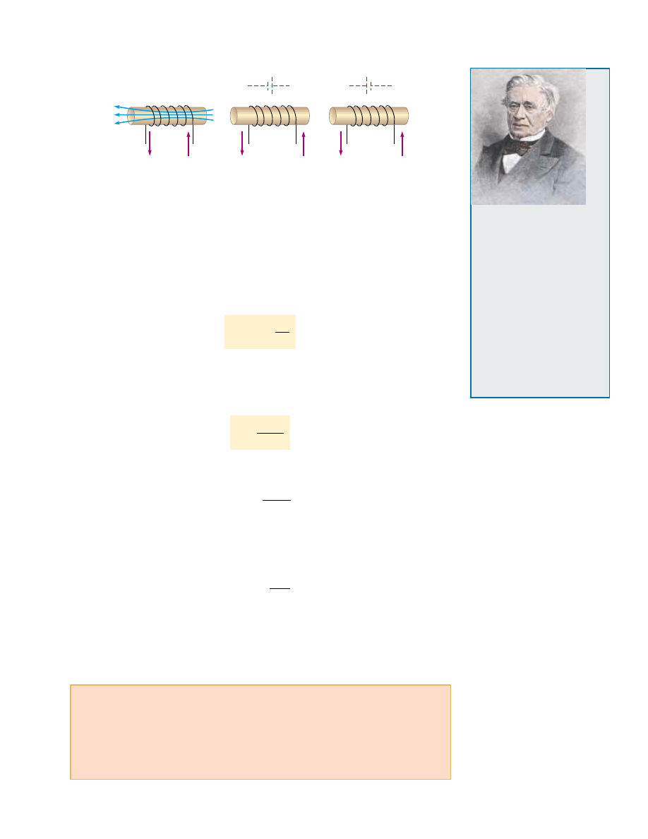
is increasing, the polarity of the induced emf is as pictured in Figure 32.2b, and if the
current is decreasing, the polarity of the induced emf is as shown in Figure 32.2c.

To obtain a quantitative description of self-induction, we recall from Faraday’s law that

the induced emf is equal to the negative of the time rate of change of the magnetic flux.
The magnetic flux is proportional to the magnetic field due to the current, which in turn
is proportional to the current in the circuit. Therefore,

a self-induced emf is always

proportional to the time rate of change of the current. For any coil, we find that

(32.1)

where L is a proportionality constant—called the

inductance of the coil—that depends

on the geometry of the coil and other physical characteristics. Combining this expression
with Faraday’s law,

" #

N d$

/dt, we see that the inductance of a closely spaced coil

of N turns (a toroid or an ideal solenoid) carrying a current I and containing N turns is

(32.2)

where it is assumed that the same magnetic flux passes through each turn.

From Equation 32.1, we can also write the inductance as the ratio

(32.3)

Recall that resistance is a measure of the opposition to current (R " %V/I ); in com-
parison, inductance is a measure of the opposition to a change in current.

The SI unit of inductance is the

henry (H), which, as we can see from Equation

32.3, is 1 volt-second per ampere:

As shown in Examples 32.1 and 32.2, the inductance of a coil depends on its geometry.
This is analogous to the capacitance of a capacitor depending on the geometry of its
plates, as we found in Chapter 26. Inductance calculations can be quite difficult to per-
form for complicated geometries; however, the examples below involve simple situa-
tions for which inductances are easily evaluated.

1 H " 1

V&s

L " #

dI/dt

L "

" #

dI
dt

Inductance of an N-turn coil

Joseph Henry

American Physicist (1797–1878)

Henry became the first director

of the Smithsonian Institution

and first president of the

Academy of Natural Science. He

improved the design of the

electromagnet and constructed

one of the first motors. He also

discovered the phenomenon of

self-induction but failed to

publish his findings. The unit of

inductance, the henry, is named

in his honor. (North Wind Picture
Archives)

Lenz’s law emf

– +

–

(a)

(b)

(c)

I increasing

I decreasing

Figure 32.2 (a) A current in the coil produces a magnetic field directed to the left.

(b) If the current increases, the increasing magnetic flux creates an induced emf in the

coil having the polarity shown by the dashed battery. (c) The polarity of the induced

emf reverses if the current decreases.

Quick Quiz 32.1

A coil with zero resistance has its ends labeled a and b. The

potential at a is higher than at b. Which of the following could be consistent with this
situation? (a) The current is constant and is directed from a to b; (b) The current is
constant and is directed from b to a; (c) The current is increasing and is directed from a
to b; (d) The current is decreasing and is directed from a to b; (e) The current is increas-
ing and is directed from b to a; (f) The current is decreasing and is directed from b to a.

Inductance

32.2 RL Circuits

If a circuit contains a coil, such as a solenoid, the self-inductance of the coil prevents
the current in the circuit from increasing or decreasing instantaneously. A circuit
element that has a large self-inductance is called an

inductor and has the circuit

symbol

. We always assume that the self-inductance of the remainder of a

circuit is negligible compared with that of the inductor. Keep in mind, however, that
even a circuit without a coil has some self-inductance that can affect the behavior of
the circuit.

Because the inductance of the inductor results in a back emf,

an inductor in a

circuit opposes changes in the current in that circuit. The inductor attempts to
keep the current the same as it was before the change occurred. If the battery voltage
in the circuit is increased so that the current rises, the inductor opposes this change,
and the rise is not instantaneous. If the battery voltage is decreased, the presence of
the inductor results in a slow drop in the current rather than an immediate drop.
Thus, the inductor causes the circuit to be “sluggish” as it reacts to changes in the
voltage.

1006

C H A P T E R 3 2 • Inductance

Example 32.1 Inductance of a Solenoid

Find the inductance of a uniformly wound solenoid having N
turns and length !. Assume that ! is much longer than the
radius of the windings and that the core of the solenoid is air.

Solution We can assume that the interior magnetic field
due to the current is uniform and given by Equation 30.17:

where n " N/! is the number of turns per unit length. The
magnetic flux through each turn is

where A is the cross-sectional area of the solenoid. Using
this expression and Equation 32.2, we find that

(32.4)

L "

BA " '

B " '

nI " '

This result shows that L depends on geometry and is propor-
tional to the square of the number of turns. Because N " n!,
we can also express the result in the form

(32.5)

where V " A! is the interior volume of the solenoid.

What If?

What would happen to the inductance if you

inserted a ferromagnetic material inside the solenoid?

Answer The  inductance  would  increase.  For  a  given
current, the magnetic flux in the solenoid is much greater
because  of  the  increase  in  the  magnetic  field  originating
from  the  magnetization  of  the  ferromagnetic  material.  For
example,  if  the  material  has  a  magnetic  permeability  of
500'

, the inductance increases by a factor of 500.

L " '

)

A " '

A! " '

Example 32.2 Calculating Inductance and emf

(A)

Calculate the inductance of an air-core solenoid con-

taining 300 turns if the length of the solenoid is 25.0 cm
and its cross-sectional area is 4.00 cm

Solution Using Equation 32.4, we obtain

0.181 mH

" 1.81 ( 10

T&m

/A "

(4) ( 10

T&m/A)(300)

(4.00 ( 10

)

25.0 ( 10

L "

(B)

Calculate the self-induced emf in the solenoid if the

current it carries is decreasing at the rate of 50.0 A/s.

Solution Using Equation 32.1 and given that dI/dt "
#

50.0 A/s, we obtain

9.05 mV

" #

(1.81 ( 10

H)(#50.0 A/s)

S E C T I O N 3 2 . 2 • RL Circuits

1007

Consider the circuit shown in Figure 32.3, which contains a battery of negligible

internal resistance. This is an

RL circuit because the elements connected to the

battery are a resistor and an inductor. Suppose that the switch S is open for t * 0 and
then closed at t " 0. The current in the circuit begins to increase, and a back emf (Eq.
32.1) that opposes the increasing current is induced in the inductor. Because the
current is increasing, dI/dt in Equation 32.1 is positive; thus,

is negative. This nega-

tive value reflects the decrease in electric potential that occurs in going from a to b
across the inductor, as indicated by the positive and negative signs in Figure 32.3.

With this in mind, we can apply Kirchhoff’s loop rule to this circuit, traversing the

circuit in the clockwise direction:

(32.6)

where IR is the voltage drop across the resistor. (We developed Kirchhoff’s rules for
circuits with steady currents, but they can also be applied to a circuit in which the
current is changing if we imagine them to represent the circuit at one instant of time.)
We must now look for a solution to this differential equation, which is similar to that
for the RC circuit. (See Section 28.4.)

A mathematical solution of Equation 32.6 represents the current in the circuit as

a function of time. To find this solution, we change variables for convenience, letting
x " (

/R) # I, so that dx " # dI. With these substitutions, we can write Equation 32.6 as

Integrating this last expression, we have

where x

is the value of x at time t " 0. Taking the antilogarithm of this result, we

obtain

Because I " 0 at t " 0, we note from the definition of x that x

/R. Hence, this last

expression is equivalent to

This expression shows how the inductor effects the current. The current does not

increase instantly to its final equilibrium value when the switch is closed but instead
increases according to an exponential function. If we remove the inductance in the
circuit, which we can do by letting L approach zero, the exponential term becomes zero
and we see that there is no time dependence of the current in this case—the current
increases instantaneously to its final equilibrium value in the absence of the inductance.

We can also write this expression as

(32.7)

I "

(1 # e

t/+

)

I "

(1 # e

Rt/L

)

I "

Rt/L

x " x

Rt/L

" #

R
L

" #

R
L

" #

R
L

x ,

L
R

IR # L

−

+
–

Active Figure 32.3 A series RL

circuit. As the current increases

toward its maximum value, an emf

that opposes the increasing current

is induced in the inductor.

At the Active Figures link

at http://www.pse6.com, you

can adjust the values of R and L

to see the effect on the current.

A graphical display as in Figure

32.4 is available.

where the constant + is the

time constant of the RL circuit:

+ "

(32.8)

Physically, + is the time interval required for the current in the circuit to reach
(1 # e

) " 0.632 " 63.2% of its final value

/R. The time constant is a useful pa-

rameter for comparing the time responses of various circuits.

Figure 32.4 shows a graph of the current versus time in the RL circuit. Note that

the equilibrium value of the current, which occurs as t approaches infinity, is

/R. We

can see this by setting dI/dt equal to zero in Equation 32.6 and solving for the current
I. (At equilibrium, the change in the current is zero.) Thus, we see that the current
initially increases very rapidly and then gradually approaches the equilibrium value

/R as t approaches infinity.

Let us also investigate the time rate of change of the current. Taking the first time

derivative of Equation 32.7, we have

(32.9)

From this result, we see that the time rate of change of the current is a maximum (equal
to

/L) at t " 0 and falls off exponentially to zero as t approaches infinity (Fig. 32.5).

Now let us consider the RL circuit shown in Figure 32.6. The curved lines on the

switch S represent a switch that is connected either to a or b at all times. (If the switch
is connected to neither a nor b, the current in the circuit suddenly stops.) Suppose that
the switch has been set at position a long enough to allow the current to reach its equi-
librium value

/R. In this situation, the circuit is described by the outer loop in Figure

32.6. If the switch is thrown from a to b, the circuit is now described by just the right
hand loop in Figure 32.6. Thus, we have a circuit with no battery (

0). Applying

Kirchhoff’s loop rule to the right-hand loop at the instant the switch is thrown from a
to b, we obtain

It is left as a problem (Problem 16) to show that the solution of this differential equa-
tion is

(32.10)

I "

t/+

IR , L

t/+

1008

C H A P T E R 3 2 • Inductance

Time constant of an RL circuit

L/R

0.632

Active Figure 32.4 Plot of the current

versus time for the RL circuit shown in

Figure 32.3. The switch is open for t * 0 and

then closed at t " 0, and the current

increases toward its maximum value

/R.

The time constant

is the time interval

required for I to reach 63.2% of its

maximum value.

Figure 32.5 Plot of dI/dt versus time for the

RL circuit shown in Figure 32.3. The time

rate of change of current is a maximum at

t " 0, which is the instant at which the switch

is closed. The rate decreases exponentially

with time as I increases toward its maximum

value.

Active Figure 32.6 An RL circuit.

When the switch S is in position a,

the battery is in the circuit. When

the switch is thrown to position b,

the battery is no longer part of the

circuit. The switch is designed so

that it is never open, which would

cause the current to stop.

At the Active Figures link

at http://www.pse6.com, you

can adjust the values of R and L

to see the effect on the current.

A graphical display as in Figure

32.7 is available.

At the Active Figures link

at http://www.pse6.com, you

can observe this graph develop

after the switch in Figure 32.3 is

closed.

Content .. 250 251 252 253 ..