Physics For Scientists And Engineers 6E - part 15

Answers to Quick Quizzes

57

Answers to Quick Quizzes

2.1 (c). If the particle moves along a line without changing di-

rection,  the  displacement  and  distance  traveled  over  any
time interval will be the same. As a result, the magnitude
of  the  average  velocity  and  the  average  speed  will  be  the
same.  If  the  particle  reverses  direction,  however,  the  dis-
placement will be less than the distance traveled. In turn,
the magnitude of the average velocity will be smaller than
the average speed.

2.2 (b). If the car is slowing down, a force must be pulling in

the direction opposite to its velocity.

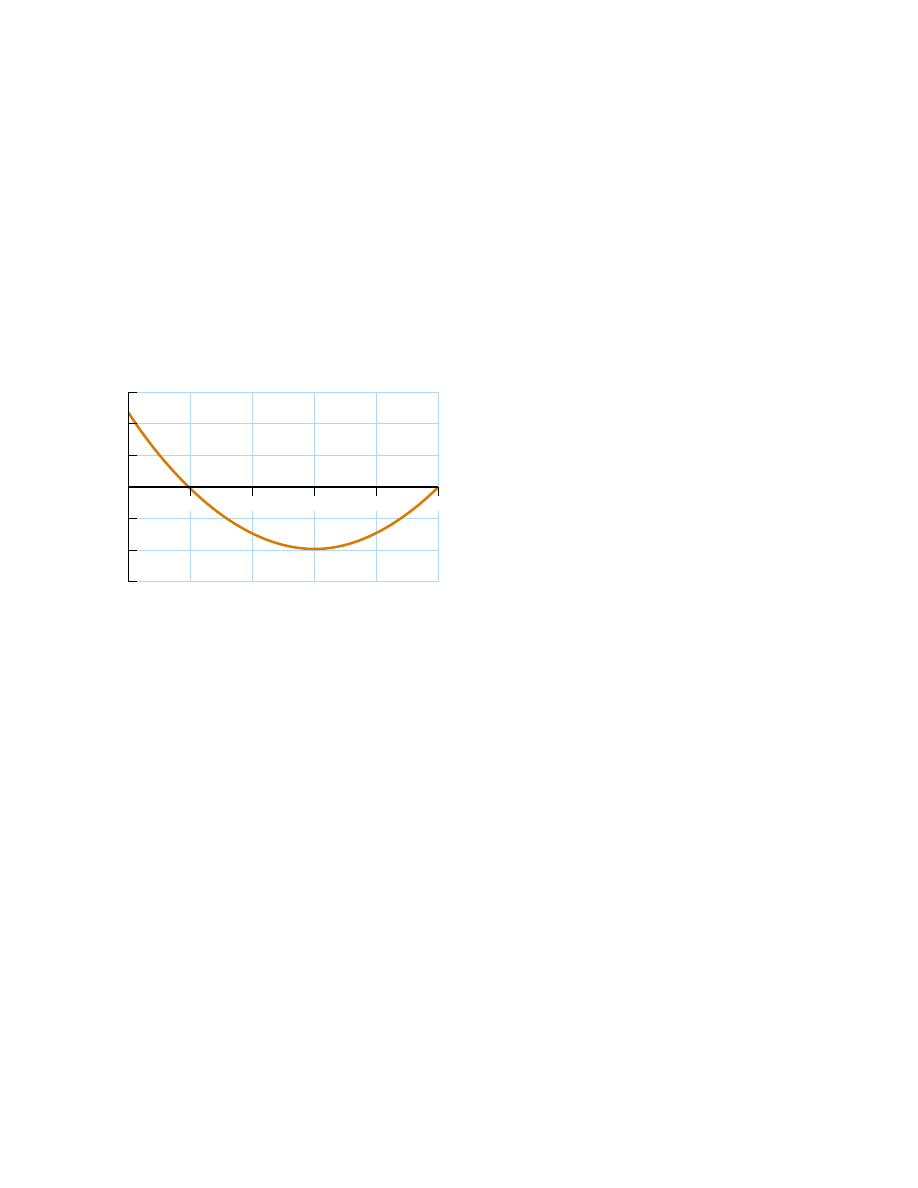
2.3 False.  Your  graph  should  look  something  like  the  follow-

ing.  This  v

x

-t graph  shows  that  the  maximum  speed  is

about 5.0 m/s, which is 18 km/h (! 11 mi/h), and so the
driver was not speeding.

2.4 (c). If a particle with constant acceleration stops and its ac-

celeration  remains  constant,  it  must  begin  to  move  again
in  the  opposite  direction.  If  it  did  not,  the  acceleration
would  change  from  its  original  constant  value  to  zero.
Choice (a) is not correct because the direction of accelera-
tion is not specified by the direction of the velocity. Choice
(b)  is  also  not  correct  by  counterexample—a  car  moving
in the # x direction and slowing down has a positive accel-
eration.

2.5 Graph (a) has a constant slope, indicating a constant accel-

eration; this is represented by graph (e).

Graph  (b)  represents  a  speed  that  is  increasing

constantly  but  not  at  a  uniform  rate.  Thus,  the
acceleration must be increasing, and the graph that best
indicates this is (d).

Graph  (c)  depicts  a  velocity  that  first  increases  at  a

constant rate, indicating constant acceleration. Then the
velocity  stops  increasing  and  becomes  constant,  indicat-
ing zero acceleration. The best match to this situation is
graph (f).

2.6 (e). For the entire time interval that the ball is in free fall,

the acceleration is that due to gravity.

2.7 (d). While the ball is rising, it is slowing down. After reach-

ing the highest point, the ball begins to fall and its speed
increases.

2.8 (a).  At  the  highest  point,  the  ball  is  momentarily  at  rest,

but still accelerating at # g.

v

x

(m/s)

t(s)

6.0

4.0

2.0

0.0

–2.0

–4.0

–6.0

20

30

40

50

10

Answer to Quick Quiz 2.3

Chapter 3

Vectors

C H A P T E R   O U T L I N E

3.1 Coordinate Systems

3.2 Vector and Scalar Quantities

3.3 Some Properties of Vectors

3.4 Components of a Vector and

Unit Vectors

58

▲

These controls in the cockpit of a commercial aircraft assist the pilot in maintaining

control over the velocity of the aircraft—how fast it is traveling and in what direction it is
traveling—allowing it to land safely. Quantities that are defined by both a magnitude and a di-
rection, such as velocity, are called vector quantities. (Mark Wagner/Getty Images)

I

n our study of physics, we often need to work with physical quantities that have both

numerical and directional properties. As noted in Section 2.1, quantities of this nature
are vector quantities. This chapter is primarily concerned with vector algebra and with
some general properties of vector quantities. We discuss the addition and subtraction
of vector quantities, together with some common applications to physical situations.

Vector quantities are used throughout this text, and it is therefore imperative that

you master both their graphical and their algebraic properties.

3.1 Coordinate Systems

Many  aspects  of  physics  involve  a  description  of  a  location  in  space.  In  Chapter  2,
for  example,  we  saw  that  the  mathematical  description  of  an  object’s  motion  re-
quires a method for describing the object’s position at various times. This descrip-
tion  is  accomplished  with  the  use  of  coordinates,  and  in  Chapter  2  we  used  the
Cartesian  coordinate  system,  in  which  horizontal  and  vertical  axes  intersect  at  a
point defined as the origin (Fig. 3.1). Cartesian coordinates are also called rectangu-
lar coordinates.

Sometimes it is more convenient to represent a point in a plane by its plane polar co-

ordinates (r, !), as shown in Figure 3.2a. In this polar coordinate system, r is the distance
from the origin to the point having Cartesian coordinates (x, y), and ! is the angle be-
tween a line drawn from the origin to the point and a fixed axis. This fixed axis is usu-
ally the positive x axis, and ! is usually measured counterclockwise from it. From the
right triangle in Figure 3.2b, we find that sin ! "

y/r and that cos ! " x/r. (A review of

trigonometric functions is given in Appendix B.4.) Therefore, starting with the plane
polar coordinates of any point, we can obtain the Cartesian coordinates by using the
equations

x " r cos !

(3.1)

y " r sin !

(3.2)

59

(–3, 4)

y

O

Q

P

(x, y)

(5, 3)

x

Figure 3.1 Designation of points in a Cartesian coor-

dinate system. Every point is labeled with coordinates

(x, y).

O

(x, y)

y

x

r

θ

(a)

θ

(b)

x

r

y

sin 

θ

 =

y

r

cos 

θ

 = xr

tan 

θ

 = x

y

θ

θ

θ

Active Figure 3.2 (a) The plane

polar coordinates of a point are

represented by the distance r and

the angle 

!

, where 

!

is measured

counterclockwise from the positive

x axis. (b) The right triangle used

to relate (x, y) to (r,

!

).

At the Active Figures link

at http://www.pse6.com, you

can move the point and see the

changes to the rectangular and

polar coordinates as well as to

the sine, cosine, and tangent of

angle 

!

.

60

CHAPTE R 3 •  Vectors

Example 3.1 Polar Coordinates

The  Cartesian  coordinates  of  a  point  in  the  xy plane  are 
(x, y) " (# 3.50, # 2.50) m, as shown in Figure 3.3. Find the
polar coordinates of this point.

Solution For  the  examples  in  this  and  the  next  two  chap-
ters we will illustrate the use of the General Problem-Solving

Strategy  outlined  at  the  end  of  Chapter  2.  In  subsequent
chapters, we will make fewer explicit references to this strat-
egy, as you will have become familiar with it and should be
applying it on your own. The drawing in Figure 3.3 helps us
to conceptualize the problem. We can categorize this as a plug-
in problem. From Equation 3.4,

and from Equation 3.3,

Note that you must use the signs of x and y to find that the
point  lies  in  the  third  quadrant  of  the  coordinate  system.
That is, ! " 216° and not 35.5°.

216$

!

 "

tan ! "

y

x

"

#

2.50 m

#

3.50 m

"

0.714

4.30 m

r "

√

x

2

%

y

2

"

√

(#3.50 m)

2

%

(#2.50 m)

2

"

(–3.50, –2.50)

x(m)

θ

r

y(m)

Active Figure 3.3 (Example 3.1) Finding polar coordinates

when Cartesian coordinates are given.

Furthermore, the definitions of trigonometry tell us that

(3.3)

(3.4)

Equation 3.4 is the familiar Pythagorean theorem.

These four expressions relating the coordinates (x, y) to the coordinates (r, !) ap-

ply only when ! is defined as shown in Figure 3.2a— in other words, when positive ! is
an angle measured counterclockwise from the positive x axis. (Some scientific calcula-
tors  perform  conversions  between  Cartesian  and  polar  coordinates  based  on  these
standard conventions.) If the reference axis for the polar angle ! is chosen to be one
other than the positive x axis or if the sense of increasing ! is chosen differently, then
the expressions relating the two sets of coordinates will change.

 r "

√

x

2

%

y

2

tan

 

! "

y

x

3.2 Vector and Scalar Quantities

As  noted  in  Chapter  2,  some  physical  quantities  are  scalar  quantities  whereas  others
are vector quantities. When you want to know the temperature outside so that you will
know how to dress, the only information you need is a number and the unit “degrees
C” or “degrees F.” Temperature is therefore an example of a scalar quantity:

A 

scalar quantity is completely specified by a single value with an appropriate unit

and has no direction.

Other examples of scalar quantities are volume, mass, speed, and time intervals. The
rules of ordinary arithmetic are used to manipulate scalar quantities.

If you are preparing to pilot a small plane and need to know the wind velocity, you

must know both the speed of the wind and its direction. Because direction is important
for its complete specification, velocity is a vector quantity: 

At the Active Figures link at http://www.pse6.com,

you can move the  point in the xy plane and see how its

Cartesian and polar coordinates change.