Intel 64 and IA-32 Architectures. Software Developer’s Manual (Collection, 2023) - page 146
9.
Updates to Chapter 20
Change bars and violet text show changes to Chapter 20 of the Intel® 64 and IA-32 Architectures Optimization
Reference Manual: Intel® Advanced Matrix Extensions (Intel® AMX).
------------------------------------------------------------------------------------------
Changes to this chapter:
•
Branding corrected throughout chapter.
•
Links and cross-references corrected throughout chapter.
•
Updated typos throughout chapter.
•
Heading Title Case Corrected throughout chapter.
•
Consolidated links throughout chapter.
•
Added and changed figure, table and example descriptions:
— Table 20-6
— Figure 20-10
— Figure 20-11
— Example 20-17
— Example 20-18
— Example 20-19
— Example 20-21
— Example 20-23
— Example 20-24
— Example 20-28
— Example 20-29
•
Section 20.1
— Updated last paragraph with new links and phrasing.
— Updated location of CPUID instruction references.
•
Section 20.5.5.3:
— Example 20-8: added space between int and m in line 2.
— Example 20-10:
• Split between two pages
• Changed
•17 _amx_interleaved_gemm_ass:
•18 amx_interleaved_gemm_ass:
•to
•17
•18 __asm {
•
Section 20.11
— Added text for clarity.
•
Section 20.16.2
— Added section about optimizing the performance of Intel® Hyper-Threading technology (Intel® HT).
Intel® 64 and IA-32 Architectures Optimization Reference Manual Documentation Changes
1313

CHAPTER 20
INTEL® ADVANCED MATRIX EXTENSIONS (INTEL® AMX)
This chapter aims to help low-level DL programmers optimally code to the metal on Intel® Xeon® Proces-
sors based on Sapphire Rapids SP microarchitecture. It extends the public documentation on Optimizing
DL code with DL Boost instructions in Section 20.8.
It explains how to detect processor support in Intel® Advanced Matrix Extensions (Intel® AMX) Architec-
ture (Section 20.1). It provides an overview of Intel AMX architecture (Section 20.2) and presents Intel
AMX instruction throughput and latency (Section 20.3). It also discusses software optimization opportu-
nities for Intel AMX (Section 20.5 through Section 20.17), TileConfig/TileRelease and compiler ABI
(Section 20.18), Intel AMX state management and system software aspects (Section 20.19), and the use
of Intel AMX for higher precision GEMMs (Section 20.20).
Table 20-1. Intel® AMX-Related Links
Description
URL
Intel® AMX architecture definitions in the Intel®
64 and IA-32 Architecture Software
Developer’s Manual
Buildable and executable templates of code
examples for this chapter.
Open VINO™ Optimization Guide
tion_guide_dldt_optimization_guide.html
oneDNN GitHub
oneDNN documentation
Intel® Optimization TensorFlow Installation
Guide
cles/guide/optimization-for-tensorflow-installation-guide.html
PyTorch Landing Page
PyTorch GitHub
Intel® Neural Compressor (INC) GitHub
Tips for measuring the performance of matrix
nical/a-simple-example-to-measure-the-performance-of-an-intel-mkl-
multiplication using Intel® MKL
function.html
Intel® AMX ABI
GitHub Repository
Using dynamically enabled XSTATE features in
Linux user space applications

INTEL® ADVANCED MATRIX EXTENSIONS (INTEL® AMX)
Table 20-1. Intel® AMX-Related Links
Description
URL
winbase-getenabledxstatefeatures
winbase-enableprocessoptionalxstatefeatures
Using dynamically enabled XSTATE features in
Windows user space applications
winbase-getthreadenabledxstatefeaturesv
threadsapi/nf-processthreadsapi-updateprocthreadattribute
20.1
DETECTING INTEL® AMX SUPPORT
Use the CPUID instruction described in Chapter 3.3 of the Intel® 64 and IA-32 Architecture Software
Developer’s Manual to find out whether the processor you are executing on supports Intel AMX at the
hardware level.
Specifically, when issuing the CPUID instruction with EAX register set to 7 and ECX register set to 0, the
instruction returns in the EDX register an indication on Intel AMX support of bits 22, 24, 25. They are all
set to 0 if Intel AMX is not supported and all set to 1 if it is supported by the processor.
Next step is check whether the OS has enabled Intel AMX state. For that you first need to issue the CPUID
instruction again to check whether the OS supports the XGETBV instruction, then use it to check whether
the OS has enabled the Intel AMX state save/restore.
When issuing the CPUID instruction with EAX register set to 1, the instruction returns an indication of
XGETBV support in bit 26 of the ECX register. If bit 26 is set, when issuing the XGETBV instruction with
ECX register set to 0, the instruction returns an indication on OS support in saving and restoring Intel
AMX state in bits 17 and 18 of the EAX register. Both bits should be set in order to use the Intel AMX
instructions. For additional CPUID information about Intel AMX, see Chapter 3.3 of the Intel® 64 and IA-
32 Architecture Software Developer’s Manual
Operating systems may require calling an OS API to allocate Intel AMX state. Visit LinuxAPI and Windows
APIs for more detailed information. Please see Section 20.19 for more information about Intel AMX state
management.
20.2
INTEL® AMX MICROARCHITECTURE OVERVIEW
General Intel AMX microarchitecture overview is available in Chapter 18 of Volume 1 of the Intel® 64 and
IA-32 Architectures Software Developer’s Manual.
20.2.1 INTEL® AMX FREQUENCIES
Discussion on the connection between max frequency, frequency license, and Instruction Set Architec-
ture covering Intel AVX technologies up to Intel® AVX-512 Instruction Set, is available in Section 2.5.3.
Intel AMX adds yet another license level whose max frequency is usually lower than that of the Intel AVX-
512 license.
When the Intel AMX unit utilization is lower than 15%, the processor may exceed the nominal max
frequency associated with Intel AMX license.
20-2

INTEL® ADVANCED MATRIX EXTENSIONS (INTEL® AMX)
20.3
INTEL® AMX INSTRUCTIONS THROUGHPUT AND LATENCY
Several Intel AMX instructions are available. Two instructions (TileLoad*) load data from the memory
hierarchy into the tile registers and one instruction (TileStore) stores the contents of a tile register into
the DCU (Data Cache Unit-first level cache). Other instructions (TDP*) execute the matrix multiplication,
operating on two input tile registers and writing the result into a third tile register. Additionally, there are
some less-frequently used instructions. The following table provides the instruction throughput and
latency counted in cycles.
Table 20-2. Intel® AMX Instruction Throughput and Latency
Instruction
Throughput
Latency
LDTILECFG
204
STTILECFG
19
TILETRELEASE
13
TDP/*
16
52
TILELOADD
8
45
TILELOADDT1
33
48
TILESTORED
16
TILEZERO
0
16
NOTE
Due to the high latency of the LDTILECFG instruction we recommend issuing a single pair
of LDTILECFG and TILERELEASE operations per Intel AMX-based DL layer implemen-
tation.
20.4
DATA STRUCTURE ALIGNMENT
GEMM and Convolution input/output data structures must be 64-byte aligned for optimal performance
but should not be aligned to 128-byte, 256-byte, etc. For more details, see Tip 6 in Tips for Measuring the
Performance of Matrix Multiplication Using Intel® MKL.
20-3
INTEL® ADVANCED MATRIX EXTENSIONS (INTEL® AMX)
20.5
GEMMS / CONVOLUTIONS
20.5.1 NOTATION
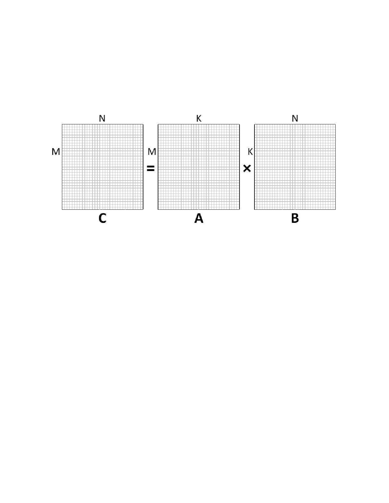
The following notation is used for the matrices (A, B, C) and the dimensions (M, K, N) in matrix multipli-
cation (GEMM).
Figure 20-1. Matrix Notation
20.5.2 TILES IN THE INTEL® AMX ARCHITECTURE
The Intel AMX instruction set operates on tiles: large two-dimensional registers with configurable dimen-
sions. The configuration is dependent on the type of tile.
• A-tiles can have between 1-16 rows and 1-MAX_TILE_K columns.
• B-tiles can have between 1-MAX_TILE_K rows and 1-16 columns.
• C-tiles can have between 1-16 rows and 1-16 columns.
MAX_TILE_K=64/sizeof(type_t), and type_t is the type of the data being operated on. Therefore,
MAX_TILE_K=64 for (u)int8 data, and MAX_TILE_K=32 for bfloat16 data. The dimensions here are
mathematical/logical. For mapping to tile register configuration parameters, see the Intel® Architecture
Instruction Set Extensions Programming Reference referenced in Section 20.2.
The type of data residing in the tiles also varies depending on the type of tile.
A tiles and B tiles contain data of type_t, which can be (u)int8 or bfloat16.
• C tiles contain data of type res_type_t:
• int32 if type_t=(u)int8
• float if type_t=bfloat16
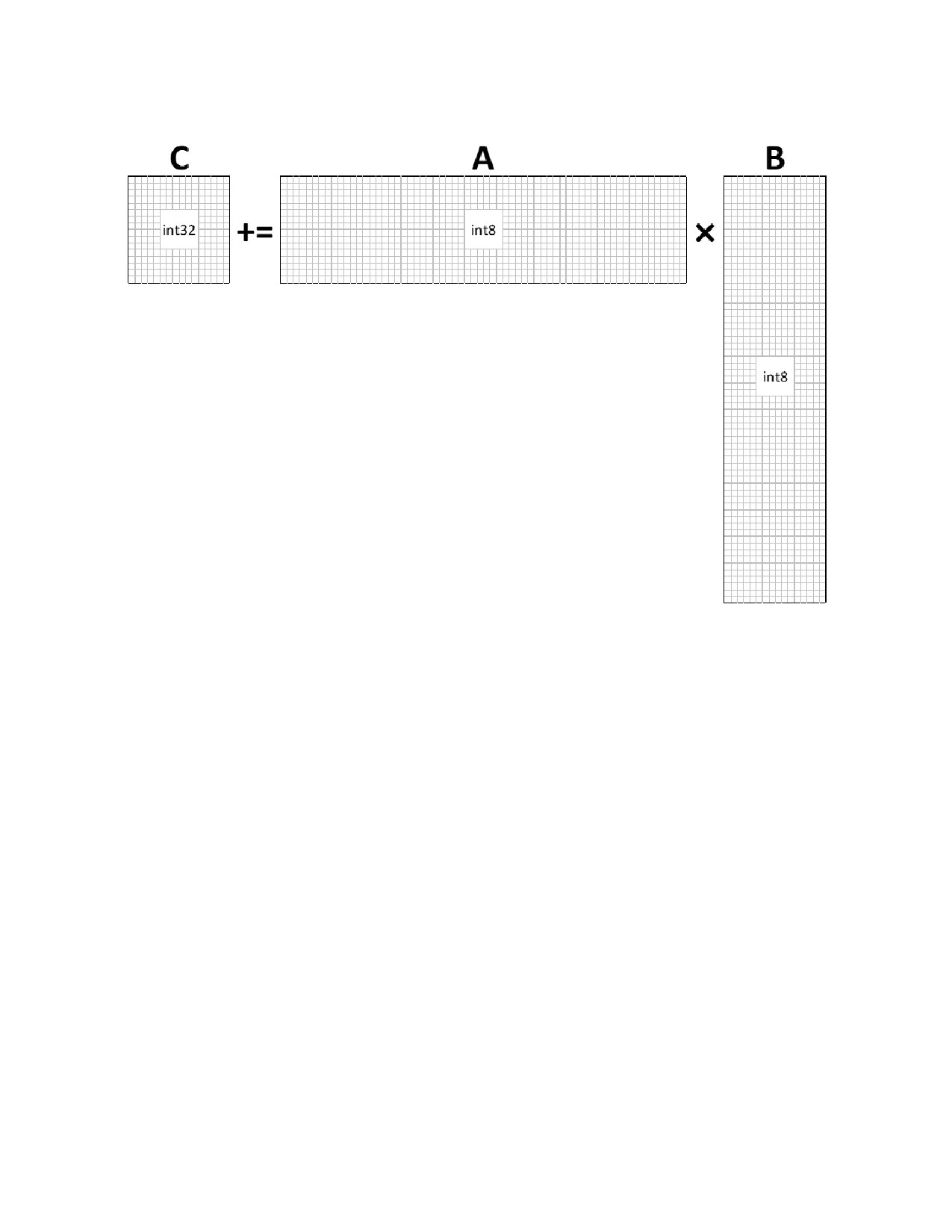
Thus, a maximum-sized tile multiplication operation for (u)int8 data type looks this way:
20-4
INTEL® ADVANCED MATRIX EXTENSIONS (INTEL® AMX)
Figure 20-2. Intel® AMX Multiplication with Max-sized int8 Tiles
TileLoad and TileStore Instructions
The tiles are loaded from memory with the TileLoad instruction and stored to memory with a TileStore
instruction. The TileLoad/TileStore instructions receive the following parameters:
• The destination/source tile of the TileLoad/TileStore.
• The source/destination location in memory for the TileLoad/TileStore.
• The stride (bytes) in memory between subsequent rows of the tile.
20-5

INTEL® ADVANCED MATRIX EXTENSIONS (INTEL® AMX)
Lines 6—10 in Example 20-1 illustrate how a tile is loaded from memory.
Example 20-1. Pseudo-Code for the Tilezero, TileLoad, and TileStore Instructions
template<size_t rows, size_t bytes_cols> class tile {
public:
friend void tilezero(tile& t) {
memset(t.v, 0, sizeof(v));
}
friend void tileload(tile& t, void* src, size_t bytes_stride) {
for (size_t row = 0; row < rows; ++row)
for (size_t bcol = 0; bcol < bytes_cols; ++bcol)
t.v[row][bcol] = static_cast<int8_t*>(src)[row*bytes_stride + bcol];
}
friend void tilestore(tile& t, void* dst, size_t bytes_stride) {
for (size_t row = 0; row < rows; ++row)
for (size_t bcol = 0; bcol < bytes_cols; ++bcol)
static_cast<int8_t*>(dst)[row*bytes_stride + bcol] = t.v[row][bcol];
}
template <class TC, class TA, class TB>
friend void tdp(TC &tC, TA &tA, TB &tB);
private:
int8_t v[rows][bytes_cols];
};
// clang-format on
template <class TC, class TA, class TB> void tdp(TC &tC, TA &tA, TB &tB)
}
For the sake of readability, a tile template class abstraction is introduced. The number of rows in the tile
and the number of column bytes per row parametrizes the abstraction.
20.5.3 B MATRIX LAYOUT
Like the Intel® DL Boost use case, the B matrix must undergo a re-layout before it can be used within the
corresponding Intel AMX multiply instruction. The re-layout procedure is as follows:
Example 20-2. B Matrix Re-Layout Procedure
#define KPACK (4/sizeof(type_t))
// Vertical K packing into Dword
type_t B_mem_orig[K][N];
// Original B matrix
type_t B_mem[K/KPACK][N][KPACK];
// Re-laid B matrix
for (int k = 0; k < K; ++k)
for (int n = 0; n < N; ++n)
B_mem[k/KPACK][n][k%KPACK] = B_mem_orig[k][n];
20-6

INTEL® ADVANCED MATRIX EXTENSIONS (INTEL® AMX)
The following figures illustrate the data re-layout process for a 64x16 int8 B matrix and a 32x16 bfloat16
B matrix (corresponding to the maximum-sized B-tile):
Figure 20-3. Re-layout of 64x16 int8 B Matrix
Figure 20-4. Re-layout of 32x16 bfloat16 B Matrix
20-7

INTEL® ADVANCED MATRIX EXTENSIONS (INTEL® AMX)
20.5.4 STRAIGHTFORWARD GEMM IMPLEMENTATION
This is GEMM reference code. Its performance is sub-optimal. Please refer to Section 20.5.5.3 for optimal
GEMM code. Begin implementation by defining the following:
Example 20-3. Common Defines
1
#define M ...
// Number of rows in the A or C matrices
2
#define K ...
// Number of columns in the A or rows in the B matrices
3
#define N ...
// Number of columns in the B or C matrices
4
#define M_ACC ...
// Number of C accumulators spanning the M dimension
5
#define N_ACC ...
// Number of C accumulators spanning the N dimension
6
#define TILE_M ...
// Number of rows in an A or C tile
7
#define TILE_K ...
// Number of columns in an A tile or rows in a B tile
8
#define TILE_N ...
// Number of columns in a B or C tile
9
10
typedef ... type_t;
// The type of data being operated on
11
typedef ... res_type_t;
// The data type of the result
12
13
#define KPACK (4/sizeof(type_t))
// Vertical K packing into Dword
14
15
type_t A_mem[M][K];
// A matrix
16
type_t B_mem[K/KPACK][N][KPACK];
// B matrix
17
res_type_t C_mem[M][N];
// C matrix
18
19
template<size_t rows, size_t bytes_cols> class tile;
20
template<class T> void tilezero (T& t);
21
template<class T> void tileload (T& t, void* src, size_t stride);
22
template<class T> void tilestore(T& t, void* dst, size_t stride);
23 template <class TC, class TA, class TB> void tdp(TC &tC, TA &tA, TB &tB) {
24
int32_t v;
25
for (size_t m = 0; m < TILE_M; m++) {
26
for (size_t k = 0; k < TILE_K / KPACK; k++) {
27
for (size_t n = 0; n < TILE_N; n++) {
28
memcpy(&v, &tC.v[m][n * 4], sizeof(v));
29
v += tA.v[m][k * 4] * tB.v[k][n * 4];
30
v += tA.v[m][k * 4 + 1] * tB.v[k][n * 4 + 1];
31
v += tA.v[m][k * 4 + 2] * tB.v[k][n * 4 + 2];
32
v += tA.v[m][k * 4 + 3] * tB.v[k][n * 4 + 3];
33
memcpy(&tC.v[m][n * 4], &v, sizeof(v));
34
}
35
}
36
}
37
}
Data type_t is the type being operated upon, i.e., signed/unsigned int8 or bfloat16. For the description of
KPACK, see Section 20.5.5. The tile template class and the three functions that operate on it are the
same as the ones introduced in Example 20-3. tilezero (t) resets the contents of tile t to 0, tileload(t, src,
stride) and loads tile t with the contents of data at src with a stride of stride between consecutive rows.
tilestore(t, dst, stride) stores the contents of tile t to dst with a stride of stride between consecutive rows.
Additionally, tdp(tC,tA,tB) performs a matrix multiplication equivalent of tC=tC+tA×tB. In reality, tiles
are defined by known compile-time integers, and the actual code operating on tiles looks slightly
different. Please visit the GitHub Repository for proper usage.
20-8

INTEL® ADVANCED MATRIX EXTENSIONS (INTEL® AMX)
The following is a simple implementation of GEMM of the matrices stored in A_mem and B_mem.
Example 20-4. Reference GEMM Implementation
for (int n = 0; n < N; n += N_ACC*TILE_N) {
for (int m = 0; m < M; m += M_ACC*TILE_M) {
tile<TILE_M, TILE_N*sizeof(res_type_t)> tC[M_ACC][N_ACC];
for (int n_acc = 0; n_acc < N_ACC; ++n_acc)
for (int m_acc = 0; m_acc < M_ACC; ++m_acc)
tilezero(tC[m_acc][n_acc]);
for (int k = 0; k < K; k += TILE_K) {
for (int n_acc = 0; n_acc < N_ACC; ++n_acc) {
tile<TILE_K/KPACK, TILE_N*KPACK> tB;
tileload(tB, B_mem[k/KPACK][n + n_acc*TILE_N], N*sizeof(type_t)*KPACK);
for (int m_acc = 0; m_acc < M_ACC; ++m_acc) {
tile<TILE_M, TILE_K*sizeof(type_t)> tA;
tileload(tA, &A_mem[m + m_acc*TILE_M][k], K*sizeof(type_t));
tdp(tC[m_acc][n_acc], tA, tB);
}
}
}
for (int n_acc = 0; n_acc < N_ACC; ++n_acc) {
for (int m_acc = 0; m_acc < M_ACC; ++m_acc) {
int mc = m + m_acc*TILE_M, nc = n + n_acc*TILE_N;
tilestore(tC[m_acc][n_acc], &C_mem[mc][nc], N*sizeof(res_type_t));
}
}
}
}
This implementation is the reference point in the following discussions.
20.5.5 OPTIMIZATIONS
20.5.5.1 Minimizing Tile Loads
Redundant tile loads may severely impact performance due to the large size of the data loaded into the
tiles, unnecessary cache evictions, etc. To minimize tile loads, it is essential to utilize the data as
completely as possible once it has been loaded into the tile.
20-9

INTEL® ADVANCED MATRIX EXTENSIONS (INTEL® AMX)
Location of the K Loop: Outside of the M_ACC and N_ACC Loops
The three loops in lines 8-18 of Example 20-4 could also have been written this way:
Example 20-5. K-Dimension Loop as Innermost Loop-A, a Highly Inefficient Approach
for (int n_acc = 0; n_acc < N_ACC; ++n_acc) {
tile<TILE_K/KPACK, TILE_N*KPACK> tB;
for (int m_acc = 0; m_acc < M_ACC; ++m_acc) {
tile<TILE_M, TILE_K*sizeof(type_t)> tA;
for (int k = 0; k < K; k += TILE_K) {
tileload(tB, B_mem[k/KPACK][n + n_acc*TILE_N], N*sizeof(type_t)*KPACK);
tileload(tA, &A_mem[m + m_acc*TILE_M][k], K*sizeof(type_t));
tdp(tC[m_acc][n_acc], tA, tB);
}
}
}
While both approaches yield correct results, there are K/TILE_K×N_ACC B tile loads in the reference
implementation. Additionally, K/TILE_K×N_ACC×M_ACC B tile loads in the implementation presented in
this section. The number of A tile loads is identical.
This approach is also characterized by excessive pressure on the memory along with an increased
number of tile loads.
Suppose the B_mem data resides in main memory. In the reference implementation, a new chunk of
TILE_K×TILE_N B data is read every M_ACC iteration of the inner loop. The inner loop then reuses the
read data. In the current implementation, when n_acc == m_acc == 0, a new chunk of TILE_K×TILE_N
B data is read every iteration of the inner loop. Then the same data is read (presumably from caches) on
subsequent iterations of n_acc, m_acc. This burst access pattern of reads from main memory results in
increased data latency and decreased performance.
Hence, keeping the K-dimension loop outside the M_ACC and N_ACC loops is recommended.
Pre-Loading Innermost Loop Tiles
Consider the following replacement code for the code in lines 8-18 of Example 20-4:
Example 20-6. Innermost Loop Tile Pre-Loading
1
for (int k = 0; k < K; k += TILE_K) {
2
tile<TILE_M, TILE_K*sizeof(type_t)> tA[M_ACC];
3
for (int m_acc = 0; m_acc < M_ACC; ++m_acc)
4
tileload(tA[m_acc], &A_mem[m + m_acc*TILE_M][k], K*sizeof(type_t));
5
for (int n_acc = 0; n_acc < N_ACC; ++n_acc) {
6
tile<TILE_K/KPACK, TILE_N*KPACK> tB;
7
tileload(tB, B_mem[k/KPACK][n + n_acc*TILE_N], N*sizeof(type_t)*KPACK);
8
for (int m_acc = 0; m_acc < M_ACC; ++m_acc) {
9
tdp(tC[m_acc][n_acc], tA[m_acc], tB);
10
}
11
}
12
}
The A-tile has been extended to an array of A-tiles (line 2) and pre-read the A tiles for the current K-loop
iteration (lines 3-4). A pre-read A-tile is used in the tile multiplication (line 9). There were
20-10

INTEL® ADVANCED MATRIX EXTENSIONS (INTEL® AMX)
K/TILE_K×N_ACC×M_ACC A-tile reads in the reference implementation, while there are only
K/TILE_K×M_ACC A-tile reads in the current implementation.
Hence, preallocation and pre-reading the tiles of the innermost loop (tA[M_ACC] in this case) is recom-
mended. The maximum number of tiles used at any given time in this scenario is
N_ACC×M_ACC+M_ACC+1 as opposed to N_ACC×M_ACC+2 in the reference implementation. Since this
optimization requires preallocation of an additional M_ACC-1 tiles, and since tiles are a scarce resource,
if N_ACC<M_ACC, it might prove beneficial to switch the order of the N_ACC and M_ACC loops. This way,
it is possible to allocate N_ACC-1<M_ACC-1 additional tiles:
Example 20-7. Switched Order of M_ACC and N_ACC Loops
for (int k = 0; k < K; k += TILE_K) {
tile<TILE_K/KPACK, TILE_N*KPACK> tB[N_ACC];
for (int n_acc = 0; n_acc < N_ACC; ++n_acc)
tileload(tB[n_acc], B_mem[k/KPACK][n + n_acc*TILE_N], N*sizeof(type_t)*KPACK);
for (int m_acc = 0; m_acc < M_ACC; ++m_acc) {
tile<TILE_M, TILE_K*sizeof(type_t)> tA;
tileload(tA, &A_mem[m + m_acc*TILE_M][k], K*sizeof(type_t));
for (int n_acc = 0; n_acc < N_ACC; ++n_acc) {
tdp(tC[m_acc][n_acc], tA, tB[n_acc]);
}
}
}
2D Accumulator Array vs. 1D Accumulator Array
Consider Example 20-6 with the following scenarios:
• N_ACC=2,M_ACC=2
• N_ACC=4,M_ACC=1
As stated before, the number of A tile loads in lines 3-11 is M_ACC, and the number of B tile loads is
N_ACC. Thus, the total number of tile loads (M_ACC+N_ACC) is 4 in the first scenario vs. 5 in the second
one (an increase of 25%), even though both scenarios perform the same amount of work.
Hence, using 2D accumulator arrays is recommended. Selecting dimensions close to square is particu-
larly recommended (since x=y minimizes f(x,y)=x+y under the constraint x×y=const).
20.5.5.2 Software Pipelining of Tile Loads and Stores
It is a best practice to interleave instructions using different resources so they may be executed in
parallel, preventing a bottleneck involving a specific resource. Therefore, preventing sequential TileLoads
and TileStores (see lines 19-23 of Example 20-4 and lines 3-4 of Example 20-6) is recommended.
Instead, interleave them with the tdp instructions (see Example 20-8).
20.5.5.3 Optimized GEMM Implementation
Below is the original code from Example 20-4, augmented with the insights from Example 20-6, with tile
loads and stores interleaved with tdps:
20-11

INTEL® ADVANCED MATRIX EXTENSIONS (INTEL® AMX)
Example 20-8. Optimized GEMM Implementation
1 for (int n = 0; n < N; n += N_ACC*TILE_N) {
2 for (int m = 0; m < M; m += M_ACC*TILE_M) {
3 tile<TILE_M, TILE_N*sizeof(res_type_t)> tC[M_ACC][N_ACC];
4 tile<TILE_M, TILE_K*sizeof(type_t)> tA[M_ACC];
5 tile<TILE_K/KPACK, TILE_N*KPACK> tB;
6
7 for (int n_acc = 0; n_acc < N_ACC; ++n_acc)
8
for (int m_acc = 0; m_acc < M_ACC; ++m_acc)
9
tilezero(tC[m_acc][n_acc]);
10
11 for (int k = 0; k < K; k += TILE_K) {
12 for (int n_acc = 0; n_acc < N_ACC; ++n_acc) {
13
tileload(tB, B_mem[k/KPACK][n + n_acc*TILE_N], N*sizeof(type_t)*KPACK);
14
for (int m_acc = 0; m_acc < M_ACC; ++m_acc) {
15
if (n_acc == 0)
16
tileload(tA[m_acc], &A_mem[m + m_acc*TILE_M][k], K*sizeof(type_t));
17
tdp(tC[m_acc][n_acc], tA[m_acc], tB);
18
if (k == K - TILE_K) {
19
int mc = m + m_acc*TILE_M, nc = n + n_acc*TILE_N;
20
tilestore(tC[m_acc][n_acc], &C_mem[mc][nc], N*sizeof(res_type_t));
21
}
22
}
23
}
24
}
25 }
26}
While placing the tile loads and stores under conditions inside the main loop (lines 13, 16, 20), conditions
can be eliminated by sufficiently unrolling the loops.
20-12

INTEL® ADVANCED MATRIX EXTENSIONS (INTEL® AMX)
The rest of this section presents a specific example of GEMM, implemented in low-level Intel AMX instruc-
tions. This is to show a full performance potential from using Intel AMX extensions.
Example 20-9. Dimension of Matrices, Data Types, and Tile Sizes
#define M 32
#define K 128
#define N 32
#define M_ACC 2
#define N_ACC 2
#define TILE_M 16
#define TILE_K 64
#define TILE_N 64
typedef int8_t type_t
typedef int32_t res_type_t
The following code is a specific example of the algorithm outlined in Example 20-8.
Example 20-10. Optimized GEMM Assembly Language Implementation
/*1 of 2*/
1
typedef struct {
2
uint8_t palette_id;
3
uint8_t startRow;
4
uint8_t reserved[14];
5
uint16_t cols[16];
6
uint8_t rows[16];
7
} __attribute__ ((__packed__)) tileconfig_t;
8
9
static const tileconfig_t tc = {
10
1,
// palette_id
11
0,
// startRow
12
0, 0, 0, 0, 0, 0, 0, 0, 0, 0, 0, 0, 0, 0,
// reserved - must be
13
64, 64, 64, 64, 64, 64, 64, 0, 0, 0, 0, 0, 0, 0, 0, 0,
// calls for 7 tiles used
14
16, 16, 16, 16, 16, 16, 16, 0, 0, 0, 0, 0, 0, 0, 0, 0
// rows for 7 tiles used
15
};
16
17
18
_asm {
19
ldtilecfg tc
# Load tile config
20
mov r8, A_mem
# Initialize register for A
21
mov r9, B_mem
# Initialize register for B
22
mov r10, C_mem
# Initialize register for C
23
24
mov r11, 128
# Initialize register for strides
25
tileloadd tmm6, [r9 + r11*1]
# Load B for n_acc = 0, k_acc = 0
26
tileloadd tmm4, [r8 + r11*1]
# Load A for m_acc = 0, k_acc = 0
27
tilezero tmm0
# Zero accumulator tile
28
tdpbssd tmm0, tmm4, tmm6
# Multiply-add tmm0 += tmm4 * tmm6
29
tileloadd tmm5, [r8 + r11*1 + 2048]
# Load A for m_acc = 1, k_acc = 0
30
tilezero tmm1
# Zero accumulator tile
20-13

INTEL® ADVANCED MATRIX EXTENSIONS (INTEL® AMX)
/*2 of 2*/
31
tdpbssd tmm1, tmm5, tmm6
# Multiply-add tmm1 += tmm5 * tmm6
32
tileloadd tmm6, [r9 + r11*1 + 64 ]
# Load B for n_acc = 1, k_acc = 0
33
tilezero tmm2
# Zero accumulator tile
34
tdpbssd tmm2, tmm4, tmm6
# Multiply-add tmm2 += tmm4 * tmm6
35
tilezero tmm3
# Zero accumulator tile
36
tdpbssd tmm3, tmm5, tmm6
# Multiply-add tmm3 += tmm5 * tmm6
37
tileloadd tmm6, [r9 + r11*1 + 2048]
# Load B for n_acc = 0, k_acc = 1
38
tileloadd tmm4, [r8 + r11*1 + 64]
# Load A for m_acc = 0, k_acc = 1
39
tdpbssd tmm0, tmm4, tmm6
# Multiply-add tmm0 += tmm4 * tmm6
40
tilestored [r10 + r11*1], tmm0
# Store C for m_acc = 0, n_acc = 0
41
tileloadd tmm5, [r8 + r11*1 + 2112]
# Load A for m_acc = 1, k_acc = 1
42
tdpbssd tmm1, tmm5, tmm6
# Multiply-add tmm1 += tmm5 * tmm6
43
tilestored [r10 + r11*1 + 2048], tmm1
# Store C for m_acc = 1, n_acc = 0
44
tileloadd tmm6, [r9 + r11*1 + 2112]
# Load B for n_acc = 1, k_acc = 1
45
tdpbssd tmm2, tmm4, tmm6
# Multiply-add tmm2 += tmm4 * tmm6
46
tilestored [r10 + r11*1 + 64], tmm2
# Store C for m_acc = 0, n_acc = 1
47
tdpbssd tmm3, tmm5, tmm6
# Multiply-add tmm3 += tmm5 * tmm6
48
tilestored [r10 + r11*1 + 2112], tmm3
# Store C for m_acc = 1, n_acc = 1
49
}
Lines 1-12 in Example 20-10 define the tile configuration for this example, and contain information about
tile sizes. Tile configuration should be loaded prior to any execution of Intel AMX instructions (line 16).
Tile sizes are defined by the configuration at the load time and can’t be changed dynamically (unless
TileRelease is called). The ‘palette_id’ field in the configuration specifies the number of logical tiles avail-
able for use; palette_id == 1 means 8 logical tiles are available, named tmm0 through tmm7. This
particular example uses 7 logical tiles (tmm4, tmm5 for A, tmm6 for B, tmm0-tmm3 for C).
According to the dimensions specified, K-loop consists of 2 iterations (cf. code listing 8.1, line 11)
according to the dimensions specified in the example. Lines 23-34 implement the first iteration and lines
35-46 the second iteration. Note the interleaving of tdp and TileStore instructions to hide the high cost of
TileStore operation.
Variable Input Dimensions
The code in Example 20-8 and 20-10 process an entire matrix of inputs of size MxK. Sometimes, only
part of the input is significant, so it is beneficial to adapt the computation to the actual input size. Often,
topologies that use self-attention it is enough to process only the first m rows of the input that are signif-
icant, where m < M. For example, taking the GEMM dimensions described above with the choice of a 1D
accumulator array of N_ACC=2,M_ACC=1, when accepting data as input with at most sixteen significant
rows, we can degenerate the m loop (line 2 in Example 20-8) so as to effectively reduce the computation
by half.
It is worth noting that in variable M dimension use cases there is an advantage to 1D accumulators. Up
to N_ACC=6, M_ACC=1 dimensions are possible if N is 96 or larger, one tile for A, one tile for B and six
tiles for the accumulator.
20.5.5.4 Direct Convolution with Intel® AMX
Direct convolution is performed directly on the input data; no data replication is required. However, there
are some layout considerations.
20-14
INTEL® ADVANCED MATRIX EXTENSIONS (INTEL® AMX)
Activations Layout
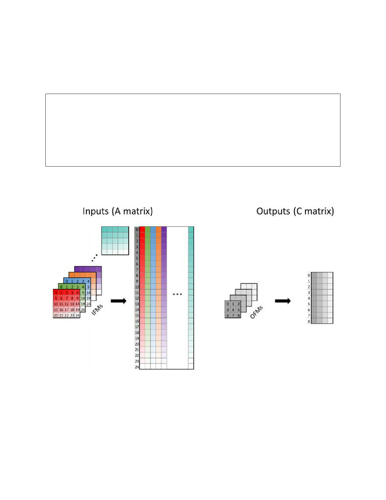
Similar to the Intel DL Boost use case, the activations are laid out in a layout obtained from the original
layout by the following procedure:
Example 20-11. Activations Layout Procedure
#define K C
// K-dimension of the A matrix = channels
#define M H*W
// M-dimension of the A matrix = spatial
type_t A_mem_orig[C][H][W];
// Original activations tensor
type_t A_mem[H][W][K];
// Re-laid A matrix7
for (int c = 0; c < C; ++c)
for (int h = 0; h < H; ++h)
for (int w = 0; w < W; ++w)
A_mem[h][w][c] = A_mem_orig[c][h][w];
This procedure on the left side of the diagram below shows the conversion of a 3-dimensional tensor into
a 2-dimensional matrix:
Figure 20-5. Activations layout
The procedure shown on the right is identical for the outputs, e.g., the activations of the next layer in the
topology).
20-15
INTEL® ADVANCED MATRIX EXTENSIONS (INTEL® AMX)
Weights Layout
Similar to the Intel DL Boost use case, the weights are re-laid by the following procedure:
Example 20-12. Weights Re-Layout Procedure
#define KH ...
// Vertical dimension of the weights
#define KW ...
// Horizontal dimension of the weights
#define KPACK (4/sizeof(type_t))
// Vertical K packing into Dword
type_t B_mem_orig[K][N][KH][KW];
// Original weights
type_t B_mem[KH][KW][K/KPACK][N][KPACK];
// Re-laid B matrices
for (int kh = 0; kh < KH; ++kh)
for (int kw = 0; kw < KW; ++kw)
for (int k = 0; k < K; ++k)
for (int n = 0; n < N; ++n)
B_mem[kh][kw][k/KPACK][n][k%KPACK] = B_mem_orig[k][n][kh][kw];
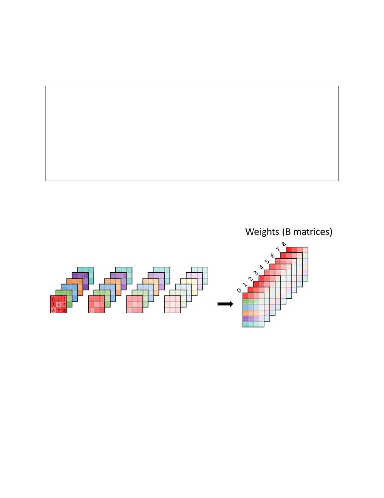
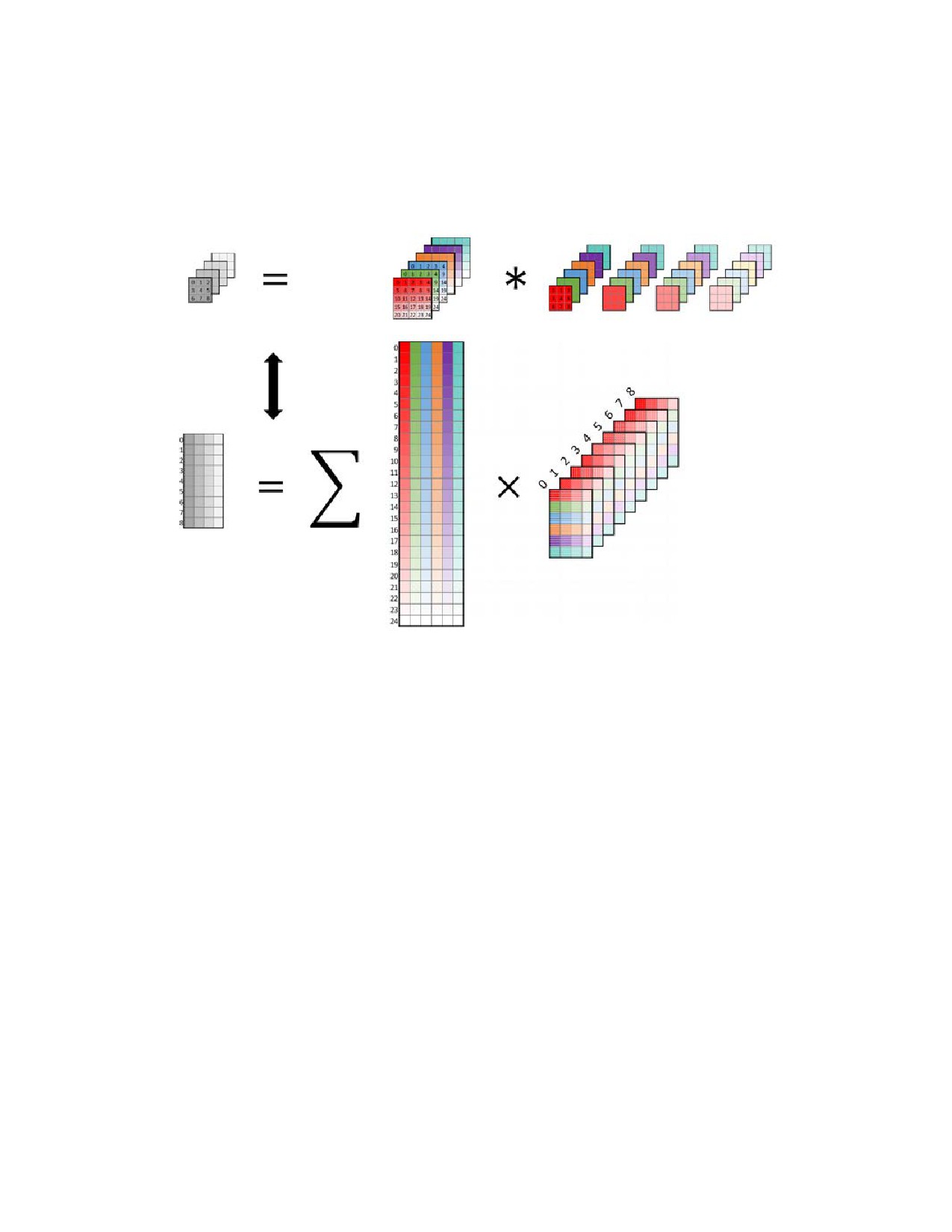
The procedure transforms the original 4-dimensional tensor into a series of 2-dimensional matrices (a
single matrix is highlighted in orange in Example 20-12) as illustrated in the following diagram for
KH=KW=3, resulting in a series of 9 B-matrices:
Figure 20-6. Weights Re-Layout
20-16
INTEL® ADVANCED MATRIX EXTENSIONS (INTEL® AMX)
20.5.5.5 Convolution - Matrix-like Multiplications and Summations Equivalence
Figure 20-7 illustrates the equivalence between convolution and summation of a series of matrix-like
multiplications between subsets of the 2-dimensional A-matrix representing the 3-dimensional activa-
tions tensor. The 2-dimensional B-matrices correspond to the various spatial elements of the weights
filter.
Figure 20-7. Convolution-Matrix Multiplication and Summation Equivalence
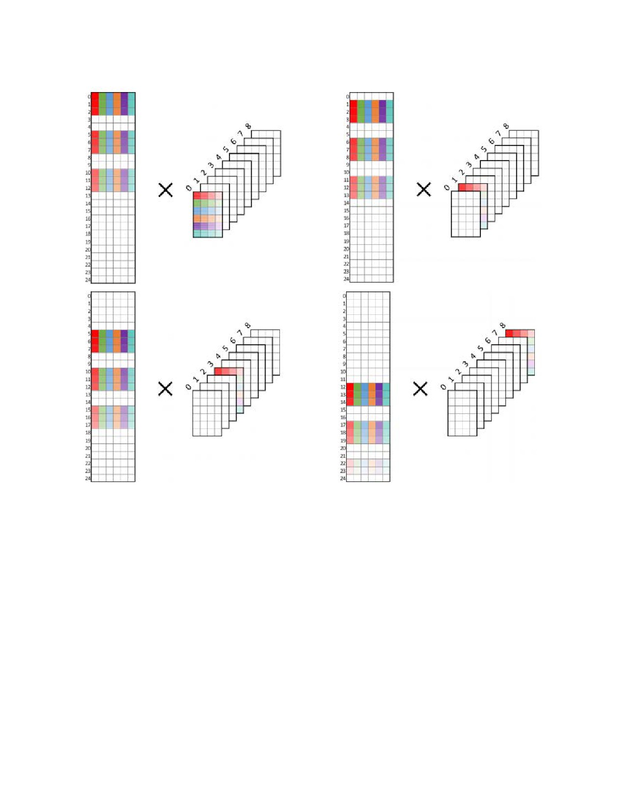
The A-matrix subset participating in the matrix-like multiplication depends on the spatial weight element
in question (i.e., the kh,kw coordinates, or the index in the range 0-8 in the previous example). For each
weight element, the A-matrix’s participating rows will interact with the weight element when the filter is
slid over the activations. For example, when sliding the filter over the activations in the previous
example, weight element 0 will only interact with activation elements 0, 1, 2, 5, 6, 7, 10, 11, and 12. For
example, it will not interact with activation element four because when the filter is applied in such a
manner (i.e., weight element 0 interacts with activation element 4), weight elements 2, 5, and 8 leave
the activation frame entirely. The A-matrix subsets for several weight elements are illustrated in the
following figure.
20-17
INTEL® ADVANCED MATRIX EXTENSIONS (INTEL® AMX)
Figure 20-8. Matrix-Like Multiplications Part of a Convolution
20-18

INTEL® ADVANCED MATRIX EXTENSIONS (INTEL® AMX)
20.5.5.6 Optimized Convolution Implementation
Replace the common defines in Example 20-3 with the following:
Example 20-13. Common Defines for Convolution
#define H ...
// The height of the activation frame
#define W ...
// The width of the activation frame
#define MA (H*W)
// The M dimension (rows) of the A matrix
#define K ...
// Number of activation channels
#define N ...
// Number of output channels
#define KH ...
// The height of the weights kernel
#define KW ...
// The width of the weights kernel
#define SH ...
// The vertical stride of the convolution
#define SW ...
// The horizontal stride of the convolution
#define M_ACC ...
// Number of C accumulators spanning the M dimension
#define N_ACC ...
// Number of C accumulators spanning the N dimension
#define TILE_M ...
// Number of rows in an A or C tile
#define TILE_K ...
// Number of columns in an A tile or rows in a B tile
#define TILE_N ...
// Number of columns in a B or C tile
#define HC ((H-KH)/SH+1)
// The height of the output frame
#define WC ((W-KW)/SW+1)
// The width of the output frame
#define MC (HC*WC)
// The M dimension (rows) of the C matrix
typedef ... type_t;
// The type of the data being operated on
typedef... res_type_t;
// The data type of the result
#define KPACK (4/sizeof(type_t))
// Vertical K packing into Dword
type_t A_mem[H][W][K];
// A matrix (equivalent to A_mem[H*W][K])
type_t B_mem[KH][KW][K/KPACK][N][KPACK];
// B matrices
res_type_t C_mem[MC][N];
// C matrix
template<size_t rows, size_t cols> class tile;
template<class T> void tilezero (T& t);
template<class T> void tileload (T& t, void* src, size_t stride);
template<class T> void tilestore(T& t, void* dst, size_t stride);
template<class TC, class TA, class TB> void tdp(TC& tC, TA& tA, TB& tB);
int mc_to_ha(int mc) {return mc / HC * SH;}
// C matrix M -> A tensor h coord
int mc_to_wa(int mc) {return mc % HC * SW;}
// C matrix M -> A tensor w coord
20-19

INTEL® ADVANCED MATRIX EXTENSIONS (INTEL® AMX)
Replace the implementation in Example 20-8 with the following:
Example 20-14. Optimized Direct Convolution Implementation
1 for (int n = 0; n < N; n += N_ACC*TILE_N) {
2 for (int m = 0; m < MC; m += M_ACC*TILE_M) {
3 tile<TILE_M, TILE_N*sizeof(res_type_t)> tC[M_ACC][N_ACC];
4 tile<TILE_M, TILE_K*sizeof(type_t)> tA[M_ACC];
5 tile<TILE_K/KPACK, TILE_N*KPACK> tB;
6
7 for (int n_acc = 0; n_acc < N_ACC; ++n_acc)
8
for (int m_acc = 0; m_acc < M_ACC; ++m_acc)
9
tilezero(tC[m_acc][n_acc]);
10
11 for (int k = 0; k < K; k += TILE_K) {
12 for (int kh = 0; kh < KH; ++kh) {
13
for (int kw = 0; kw < KW; ++kw) {
14
for (int n_acc = 0; n_acc < N_ACC; ++n_acc) {
15
int nc = n + n_acc*TILE_N;
16
tileload(tB, B_mem[kh][kw][k/KPACK][nc], N*sizeof(type_t)*KPACK);
17
for (int m_acc = 0; m_acc < M_ACC; ++m_acc) {
18
int mc = m + m_acc*TILE_M;
19
if (n_acc == 0) {
20
int ha = mc_to_ha(mc)+kh, wa = mc_to_wa(mc)+kw;
21
tileload(tA[m_acc], &A_mem[ha][wa][k], K*SW*sizeof(type_t));
22
}
23
tdp(tC[m_acc][n_acc], tA[m_acc], tB);
24
if (k + kh + kw == K - TILE_K + KH + KW - 2)
25
tilestore(tC[m_acc][n_acc], &C_mem[mc][nc], N*sizeof(res_type_t));
26
}
27
}
28
}
29
}
30
}
31 }
32 }
The divergences highlighted in yellow in Example 20-8 include:
• The loop over M-dimension (line 2) references the M-dimension of the C-matrix (since the M-
dimensions of A and C no longer have to be the same). To get the corresponding A-matrix m index
from a C-matrix m index, one must employ the conversion functions mc_to_ha() and mc_to_wa()
(line 20).
• There are additional loops over the weights kernel dimensions KH and KW (lines 12-13), which define
the B-matrix to be used (line 16), enter into the condition for accumulator tile storing (line 24) and
computation of A-matrix coordinates (line 20).
• The stride of the A tile load must account for the convolutional horizontal stride (line 21).
Note that care should be taken to define TILE_M*M_ACC in such a way that it cleanly divides WC (the
width of the output frame), i.e., WC%(TILE_M*M_ACC)==0. Otherwise, some tiles will end up loading
data that should not be multiplied by the corresponding weight element (see Figure 20-8). Possible miti-
gations of this issue:
• An M_ACC loop with a dynamic upper limit depending on the current position in A.
20-20

INTEL® ADVANCED MATRIX EXTENSIONS (INTEL® AMX)
• Use different sized A tiles (and correspondingly C tiles) depending on the current position in A (if
there are enough free tiles, performing TileConfig during the convolution is highly discouraged).
• Define TILE_M without consideration for WC and remove/disregard the “junk” data from the results at
the post-processing stage (code not shown). Care should be taken in this case concerning the
advancement of the m index (line 2) since the current assumption is that every row of every tile is
valid (corresponds to a row in the C matrix). If “junk” data is loaded, this is no longer the case: a C-
tile will have less than TILE_M rows of C.
Location of the KH, KW Loops
As shown in Example 20-5, it is ill-advised to put the loop over the K-dimension inside an inner M_ACC or
N_ACC loop. The same considerations hold in the case of the kh,kw loops. While there is no functional
obstacle precluding the positioning of the kh,kw loops further up (before lines 12-13), it is recommended
to keep them under the K loop and above the M_ACC, N_ACC loops because, during the traversal of
kh,kw with the same k value, the TileLoad of A-data (line 21) will have much overlap with A-data loaded
for previous values of kh,kw (with the same k value). This data will likely reside in the lowest-level cache.
Moving the kh,kw loops upward will reduce that likelihood.
20.6
CACHE BLOCKING
Data movement costs vary greatly depending on where the data lies in the cache hierarchy. When the
matrices involved in a GEMM or convolution are larger than the available cache, computations must
proceed in such a manner as to optimize data reuse from the cache. Here a simple cache-blocking
scheme is implemented to simultaneously process partial blocks of the A, B, and C matrices.
20.6.1 OPTIMIZED CONVOLUTION IMPLEMENTATION WITH CACHE BLOCKING
In the following example, the focus is on implementing cache blocking for the optimized convolution
implementation described in the Optimized Convolution Implementation <XREF> section. However, note
that similar changes can also be made to the optimized GEMM implementation. Alternatively, the GEMM
implementation can be derived as a special case of convolution with KH=KW=1 and SH=SW=1.
In addition to the common defines in Example 20-13, add the following:
Example 20-15. Additional Defines for Convolution with Cache Blocking
#define MC_CACHE ...
// Extent of cache block along the M dimension of the C matrix
#define K_CACHE ...
// Extent of cache block along the K dimension
#define N_CACHE ...
// Extent of cache block along the N dimension
typedef ... acc_type_t;
// The accumulation data type (either int32 or float)
acc_type_t aC_mem[M_ACC][N_ACC][TILE_M][TILE_N];
// Accumulator buffers of C
20-21

INTEL® ADVANCED MATRIX EXTENSIONS (INTEL® AMX)
Replace the implementation in Example 20-14 with the following:
Example 20-16. Optimized Convolution Implementation with Cache Blocking
1 for (int nb = 0; nb < N; nb += N_CACHE) {
2 for (int mb = 0; mb < MC; mb += MC_CACHE) {
3 for (int kb = 0; kb < K; kb += K_CACHE) {
4
for (int n = nb; n < nb + N_CACHE; n += N_ACC*TILE_N) {
5
for (int m = mb; m < mb + MC_CACHE; m += M_ACC*TILE_M) {
6
tile<TILE_M, TILE_N*sizeof(res_type_t)> tC[M_ACC][N_ACC];
7
tile<TILE_M, TILE_K*sizeof(type_t)> tA[M_ACC];
8
tile<TILE_K/KPACK, TILE_N*KPACK> tB;
9
10
for (int n_acc = 0; n_acc < N_ACC; ++n_acc)
11
for (int m_acc = 0; m_acc < M_ACC; ++m_acc)
12
if (kb == 0)
13
tilezero(tC[m_acc][n_acc]);
14
else {
15
int m_aC = (m - mb) / TILE_M + m_acc;
16
int n_aC = (n - nb) / TILE_N + n_acc;
17
tileload(tC[m_acc][n_acc], &aC_mem[m_aC][n_aC],
18
TILE_N*sizeof(acc_type_t));
19
}
20
21
for (int k = kb; k < kb + K_CACHE; k += TILE_K) {
22
for (int kh = 0; kh < KH; ++kh) {
23
for (int kw = 0; kw < KW; ++kw) {
24
for (int n_acc = 0; n_acc < N_ACC; ++n_acc) {
25
int nc = n + n_acc*TILE_N;
26
tileload(tB, B_mem[kh][kw][k/KPACK][nc], N*sizeof(type_t)*KPACK);
27
for (int m_acc = 0; m_acc < M_ACC; ++m_acc) {
28
int mc = m + m_acc*TILE_M;
29
if (n_acc == 0) {
30
int ha = mc_to_ha(mc)+kh, wa = mc_to_wa(mc)+kw;
31
tileload(tA[m_acc], &A_mem[ha][wa][k], K*SW*sizeof(type_t));
32
}
33
tdp(tC[m_acc][n_acc], tA[m_acc], tB);
34
if (k + kh + kw == K - TILE_K + KH + KW - 2)
35
tilestore(tC[m_acc][n_acc], &C_mem[mc][nc],
36
N*sizeof(res_type_t));
37
else if (k + kh + kw == kb + K_CACHE - TILE_K + KH + KW - 2) {
38
int m_aC = (m - mb) / TILE_M + m_acc;
39
int n_aC = (n - nb) / TILE_N + n_acc;
40
tilestore(tC[m_acc][n_acc], &aC_mem[m_aC][n_aC],
41
TILE_N*sizeof(acc_type_t));
42
}
43
}
44
}
45
}
46
}
47
}
48
}
49
}
50
}
51 }
52 }
20-22

INTEL® ADVANCED MATRIX EXTENSIONS (INTEL® AMX)
The loops over the N, MC, and K dimensions are replaced by loops over cache blocks of N, MC, and K.
Additional loops over the entire N, MC, and K-dimensions are added at the outermost level. These loops
have a step size equal to the cache blocks of N, MC, and K.
In the case of cache blocking along the K-dimension, additional calls to TileLoad and TileStore are
required to load and store intermediate accumulation results. Note that this adds additional memory
traffic, especially for int8 output data types (as Accumulation data type is either int32_t or float). For this
reason, it is generally not advisable to block along the K dimension.
For simplicity, assume the following relationships:
• N is an integer multiple of N_CACHE: an integer multiple of N_ACC*TILE_N.
• MC is an integer multiple of MC_CACHE: an integer multiple of M_ACC*TILE_M. As before, the
condition WC%(TILE_M*M_ACC)==0 still holds.
• K is an integer multiple of K_CACHE: an integer multiple of TILE_K.
Define the following set of operations as the compute kernel of the optimized convolution implementa-
tion. First, initialize the accumulation tiles to zero (line 13) for an M_ACC*TILE_M x N_ACC*TILE_N
chunk of the C-matrix. Next, for each of the KH*KW B-matrices, the matrix multiplication of the corre-
sponding M_ACC*TILE_M x K chunk of the A-matrix by a K x N_ACC*TILE_N chunk of the B-matrix is
performed, each time accumulating to the same set of accumulation tiles (lines 18-30). Finally, the
results are stored in the C-matrix (line 32).
Continue with the computation of a full cache block of C-matrix, ignoring any blocking along the K-
dimension. First, the kernel is performed for the first chunks of the A, B, and C cache blocks. Next, the
chunks of A and C advance along the M dimension, and the kernel is repeated with the same chunk set of
the B-matrices. The above step is repeated until the last chunks of A and C in the current cache block
have been accessed. Next, the chunks of B and C are advanced along the N-dimension by N_ACC*TILE_N
and the chunk of A returns to the beginning of its cache block.
Observe the following from the above description of the computation of a full cache block of the C-
matrix:
• For each kernel iteration, it is better if the current chunk of matrix A (roughly
KH*M_ACC*TILE_M*K*sizeof(type_t)) fits into the DCU. This allows for maximal data reuse between
the partially overlapping regions of A that need to be accessed by the different B matrices.
• Advancing from one chunk of matrix A to the next, it is better if the current chunk set of the B
matrices (in total, KH*KW*K*N_ACC*TILE_N*sizeof(type_t)) fits into the DCU.
• Advancing from one chunk set of the B matrices to the next, it is better if the current cache block of
matrix A fits into the MLC.
• Advancing from one cache block of matrix A to the next, it is better if the current cache block of the
B matrices (in total, KH*KW*K*N_CACHE*sizeof(type_t)) fits into the MLC.
From these observations, a general cache blocking strategy is choosing MC_CACHE and N_CACHE to be as
large as possible while keeping the A, B, and C cache blocks in the MLC.
Intel® AMX-Specific Considerations
A specific feature of Intel AMX-accelerated kernels to keep in mind when applying the previous cache-
blocking recommendations is any post-processing of results from the Intel AMX unit (e.g., adding bias,
dequantizing, converting between data types) must occur by way of vector registers. Thus, a buffer is
needed to store results from the accumulation tiles and load them into vector registers for post-
processing. Note that if acc_type_t is the same as res_type_t, the C matrix itself can be used to store
intermediate results. However, the buffer is small (at most 4KB for the accumulation strategies described
in vSection ) and easily fits into the DCU. While it should still be considered when determining the optimal
cache block partitioning, it is unlikely to influence kernel performance strongly.
20-23
INTEL® ADVANCED MATRIX EXTENSIONS (INTEL® AMX)
20.7
MINI-BATCHING IN LARGE BATCH INFERENCE
Layers have different sizes and shapes, which require different cache and memory-blocking strategies.
There are layers with a small spatial dimension (M) and relatively larger shared dimension (K) and SIMD
dimension (N). In such layers, the weights are significantly larger than the inputs. Therefore, most of the
load operations are weights matrix loads whose cost is high when the weights reside in memory or the
last level cache.
Running a large batch allows employing an optimization that amortizes the cost of loading the weight
matrix. The idea is to use the same weights for multiple inputs, e.g., execute the same layer with multiple
images. This optimization is highly applicable in CNNs where the inputs of the first layers are large while
the weights are relatively small but end with small input images and large weight matrices. Optimal
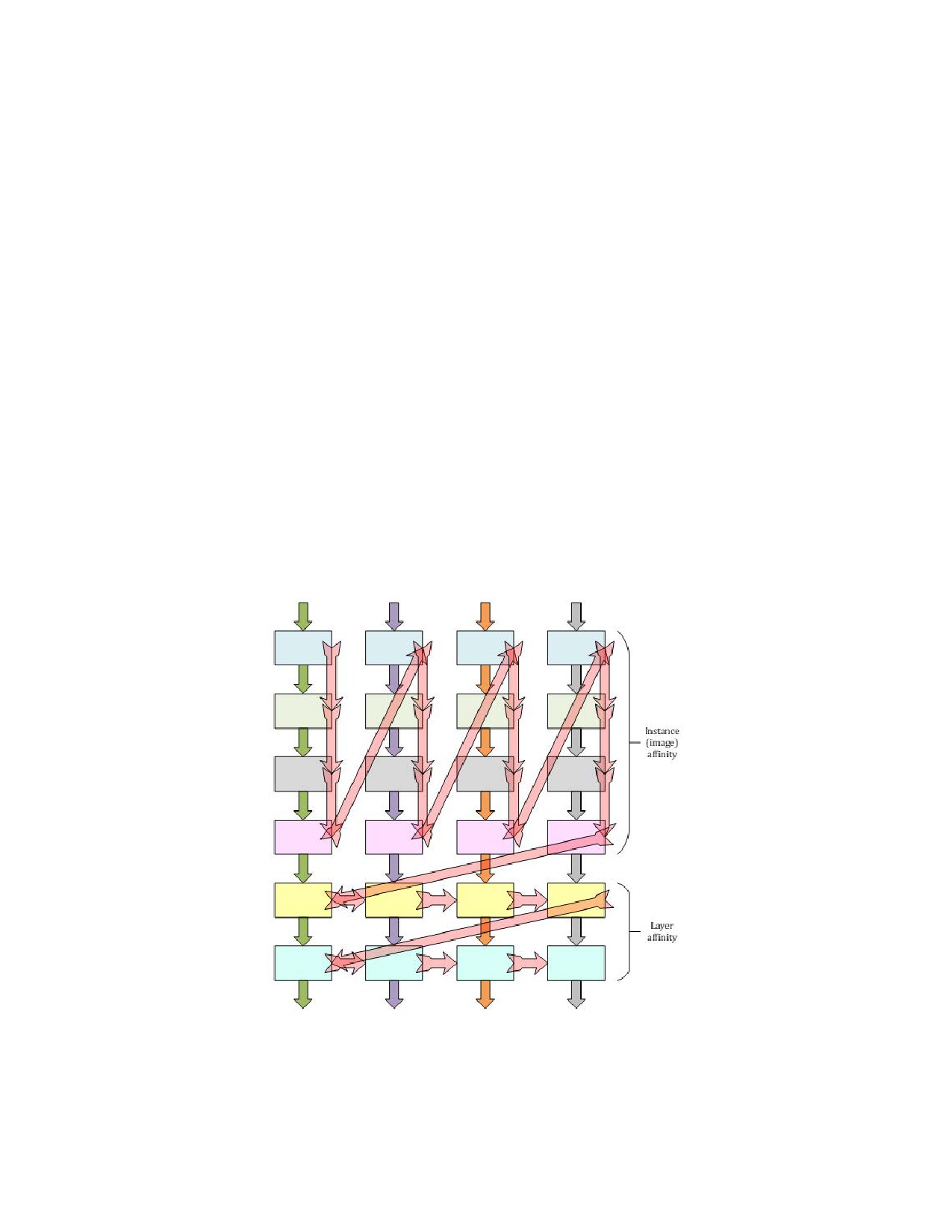
execution of the topology starts in the instance or image affinity, where a single input goes through one
layer after another before the next input is retrieved. At some point, the topology execution switches to
layer affinity, where the same layer processes several inputs (mini-batch) before moving forward to the
next layer.
For example, in ResNet-50, the conv-1 to conv-4 layers have relatively large IFMs and smaller weight
matrices. However, many weight matrices are larger than MLC size (mid-level cache) in the conv-5
layers. The switchover point from image affinity to layer affinity on a 4th Generation Intel® Xeon®
Processor microarchitecture is the first layer of conv-5.
The diagram below illustrates six layers with four instances per thread (mini-batch of four). Boxes with
identical colors identify the same layers in each column. Arrows flowing downward through each column’s
layers represent the data flow of a particular instance. Translucent red arrows identify the execution
order of layers with corresponding instances. The first four layers of the diagram have instance (aka
image) affinity, and the last two have layer affinity.
Figure 20-9. Batching Execution Using Six Layers with Four Instances Per Thread
On Resnet-50, this optimization can yield a 17% performance gain.
20-24

INTEL® ADVANCED MATRIX EXTENSIONS (INTEL® AMX)
20.8
NON-TEMPORAL TILE LOADS
When a regular tile load is issued, the data for the tile are placed in L2, L1, and then in the tile register
(DRAM/L3->L2->L1->tile register), as with any other register load. This has the well-known benefit of
reduced data read latency due to data proximity when recently accessed data are reaccessed after a
short time. However, indiscriminate application of this approach might sometimes prove detrimental.
Consider the code in Example 20-4, referring to the unoptimized, unblocked implementation for
simplicity. The five loops in the code listing alongside the total input (A) matrix data and weights (B)
matrix data accessed at each loop level is shown in the following table. The original row in the code listing
is provided for convenience:
Table 20-3. Five Loops in Example 20-4
Row
Var
Variable Range
A Data Size
B Data Size
1
n
[0:N:N_ACC×TILE_N]
M×K
K×N
2
m
[0:M:M_ACC×TILE_M]
M×K
K×N_ACC×TILE_N
8
k
[0:K:TILE_K]
MC_CACHE×K
9
n acc
[0:N_ACC:1]
M_ACC×TILE_M×TILE_K
TILE_K×N_ACC×TILE_N
12
m ac
[0:M_ACC:1]
20.8.1 PRIORITY INVERSION SCENARIOS WITH TEMPORAL LOADS
For the following discussion, assume:
• The data type is int8 (i.e., each element in the table above takes 1 byte).
• TILE_M=16, TILE_K=64, TILE_N=16 (i.e., all tiles are of size 1kB).
• L1 cache size is 32kB.
• M_AC=N_ACC=2.
Scenario One:
Consider the following scenario, including M=256, K=1024, and N=256.
Table 20-4 illustrates accessed data sizes:
Table 20-4. Accessed Data Sizes: Scenario One
Row
Var
Variable Range
A Data Size
B Data Size
1
n
[0:N:N_ACC×TILE_N]
256kB
256kB
2
m
[0:M:M_ACC×TILE_M]
32kB
8
k
[0:K:TILE_K]
32kB
9
n acc
[0:N_ACC:1]
32kB
2kB
12
m ac
[0:M_ACC:1]
At the k loop level, the combined sizes of A and B accessed data will overflow the L1 cache by a factor of
two. Proceeding to the m-level since m is progressing, new A-data are constantly read (a total of 256kB-
32kB=224kB new A data), while the same 32kB of B data are being accessed repeatedly. Thus, a priority
inversion occurs: new A-data placed in the L1 cache repeatedly are accessed only once. They evict the
32kB of B data that are accessed eight times. Placement of A data in the L1 cache is not beneficial: the
20-25

INTEL® ADVANCED MATRIX EXTENSIONS (INTEL® AMX)
next time the same data are accessed will be in the n loop after 256kB (x8 L1 cache size) of A data has
been read. Additionally, it is detrimental because it causes repeated eviction of 32kB of B data that could
have been read from the L1 cache eight times.
Scenario Two:
Consider the following scenario, including M=32, K=1024, and N=256. Here, the M-dimension is covered
in the m_acc loop, and the loop over m is redundant. The priority inversion is: as n advances, new B-data
(accessed only once) repeatedly evict 32kB of A-data that could have been read (8 times) from the L1
cache had it not been pushed out by B-data.
Here, the M-dimension is covered in the m_acc loop, and the loop over m is redundant. The priority
inversion is: as n advances, new B-data (accessed only once) repeatedly evict 32kB of A-data that
could have been read (8 times) from the L1 cache had it not been pushed out by B-data.
Table 20-5. Accessed Data Sizes: Scenario Two
Row
Var
Variable Range
A Data Size
B Data Size
1
n
[0:N:N_ACC×TILE_N]
256kB
2
m
[0:M:M_ACC×TILE_M]
32kB
32kB
8
k
[0:K:TILE_K]
9
n acc
[0:N_ACC:1]
2kB
2kB
12
m ac
[0:M_ACC:1]
These two basic scenarios can be readily extended to the blocked code in Example 20-16.
Table 20-6. Accessed Data Sizes Extended to Blocked Code
Row
Var
Variable Range
A Data Size
B Data Size
1
nb
[0:N:N_CACHE]
M×K
2
mb
[0:MC:MC_CACHE]
M×K
3
kb
[0:K:K_CACHE]
MC_CACHE×K
4
n
[nb:nb+N_CACHE:N_ACC×TILE_N]
K_CACHE×KH×KW×N_ACC×TILE_
5
m
[mb:mb+MC_CACHE:M_ACC×TILE_M]
MC_CACHE×K_CACHE
N
18
k
[kb:kb+K_CACHE:TILE_K]
19
kh
[0:KH:1]
/*/*
TILE_K×KH×KW×N_ACC×TILE_N
20
kw
[0:KW:1]
21
n acc
[0:N_ACC:1]
M_ACC×TILE_M×TILE_K
TILE_K×N_ACC×TILE_N
24
m ac
[0:M_ACC:1]
NOTE
Due to the nature of convolution, the loops over kh, kw reuse most of the A-data.
The innermost loops m_acc, n_acc, kh,kw will access at most M_ACC kB of A data and KH×KW×N_ACC
kB of B-data, which, in some cases (e.g., KH=KW=3, N_ACC=4) might already overflow the L1 cache
size. Thus, several opportunities for priority inversions exist in this more complex loop structure,
depending on the parameters in the table above:
20-26
INTEL® ADVANCED MATRIX EXTENSIONS (INTEL® AMX)
• B-data evicting reusable A-data at the kh,kw loops level.
• A-data evicting reusable B-data at the m loop level.
• B-data evicting reusable A-data at the n loop level.
• A-data evicting reusable B-data at the mb loop level.
• B-data evicting reusable A-data at the nb loop level.
Solution to Priority Inversions: Non-Temporal Loads
Intel AMX architecture introduces a way to load tile registers bypassing the L1 cache via non-temporal
tile loads (TILELOADDT1). This allows the user to deal with priority inversions such as those described
above by loading the large, non-reusable data chunk with non-temporal loads. Thus, the larger chunk is
prevented from evicting the smaller, frequently used data chunk. In Table 20-4, the A-tiles are loaded
with non-temporal loads while loading B-tiles with temporal loads. This ensures the B-tile loads at the m
loop level will all come from the L1 cache. In Table 20-5, the B-tiles are loaded with non-temporal loads
while loading A-tiles with temporal loads, thus ensuring that the A-tile loads at the n loop level will all
come from the SL1 cache.
20.9
USING LARGE TILES IN SMALL CONVOLUTIONS TO MAXIMIZE DATA
REUSE
A convolution with a small-sized input frame can make the Intel AMX computation inefficient.
Consider the following example: a 7x7 input frame, with padding of 1 (size including padding is 9x9),
convolved with a 3x3 filter to produce a 7x7 output frame.
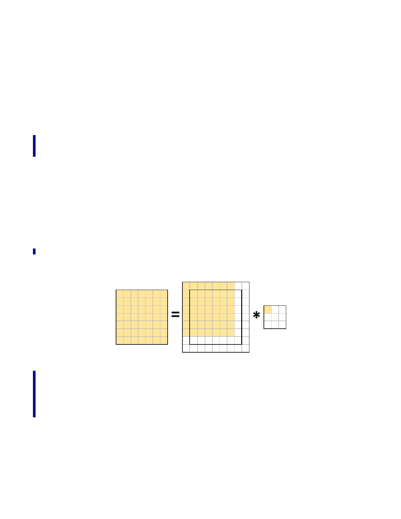
Figure 20-10 shows the pieces participating in the convolution (in yellow) interacting with the khaki=0,0
weight element.
Figure 20-10. A Convolution Example
Thus, the yellow parts of the input frame are the only ones that should be loaded into A-tiles when
processing weight element kh,kw=0,0. The white parts of the input frame should be ignored. This
requires the number of tile rows to be set at seven, utilizing less than half of the A-tile, reducing B
(weights) data reuse by a factor of two. Each A-tile is now half the size, and seven tiles are required to
cover the spatial dimension. Because there are not seven tiles, B-tiles must be loaded twice as many
times, potentially leading to significant performance degradation, depending on the size of the weights.
This is usually inversely proportional to the spatial size of the input frame).
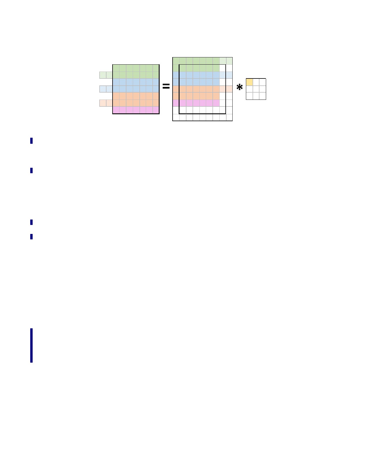
Figure 20-11 shows three A-tiles with sixteen rows and one tile with seven rows to cover the entire
spatial dimension of the convolution.
20-27
INTEL® ADVANCED MATRIX EXTENSIONS (INTEL® AMX)
Figure 20-11. A Convolution Example with Large Tiles.
Each tile is highlighted differently. The green, blue, and orange tiles now load those two “extra” pieces
previously ignored. Those pieces will waste compute resources and take up two rows in the accumulator
tiles. The user may choose to ignore those rows in subsequent computations (e.g., int8-quantization,
RELU, etc.), complicating the implementation. The potential benefit of increased B-data reuse could be
dramatic, however.
20.10 HANDLING INCONVENIENTLY-SIZED ACTIVATIONS
Occasionally, the spatial dimensions of an activation might be ill-suited for efficient tiling with tiles.
Consider a GEMM with activations’ M=100. This poses a challenge: while the M dimension can be neatly
tiled by ten tiles, each with ten rows, this approach is inefficient since a larger M dimension of 112
requires only seven tiles with sixteen rows. This means that the data reuse for M=100 is 30% worse than
for M=112.
The following solutions will be useful:
1. Define two types of A- and C-tiles - tiles with 16 rows and one tile with four. Use tiles of the first type
for M=0..9 and the second type tile for M=96..99.
2. Allocate extra space in A and C buffers, as if M=112, and use tiles with 16 rows exclusively. The extra
space need not be zeroed out or otherwise prepared in any way. In this case, the last (seventh) tile
will load four meaningful rows (M=96..99) and twelve “garbage” rows (M=100..111). At the output,
tile C will have four meaningful rows (M=96..99) and twelve “garbage” rows (M=100..111) which the
user can then ignore.
The first solution does not require tampering with the A and C buffers and computes 100 tile rows,
producing a clean result. Still, it requires additional A- and C-tiles. unused throughout the computation
except at the very end. Since only eight tiles are available, this requirement can be costly and might
reduce the data reuse (e.g., to use a 2D accumulator array, you would need three x2 C-tiles, two A-tiles,
and two B-tiles, equaling ten tiles). The second solution avoids this requirement by complicating buffer
handling and paying with additional loads, compute, and storing (it loads, computes, and stores 112 tile
rows).
20-28

INTEL® ADVANCED MATRIX EXTENSIONS (INTEL® AMX)
20.11 POST-CONVOLUTION OPTIMIZATIONS
Most Intel AMX-friendly applications are from the Deep Learning domain, where the data flows through
multiple layers. It is often necessary to process the convolution output before passing it as an input to the
next layer (processing operations depend on a specific application). This stage is called post-convolu-
tion.
20.11.1 POST-CONVOLUTION FUSION
As with Intel AVX-512 code, a critical optimization is the “fusion” of post-convolutional operations to the
convolutional data they operate upon. Fusion reduces the memory hierarchy thrashing. Additionally,
fusing the quantization step gains x2 (for bfloat16 data type) or x4 (for int8 data type) compute band-
width, and reduces memory bandwidth by x2 or x4, respectively.
Consider the code in Example 20-8. Lines 7-24 contain the entire GEMM operation for any M, N coordi-
nate in the output. Thus, the optimal location to post-process the data computed in lines 7-24 is right
before line 24 while it is still in the low-level cache.
In Example 20-17, blue code illustrates a fully unrolled example from line 7 through 24, for int8 GEMM
with K=192, N_ACC=M_ACC=2, TILE_M=2, TILE_K=64, TILE_N=16. The convolution code is fused with
post-convolution code (blue) that quantizes the output and ReLU. To keep the post-convolution code in
the example short, an unrealistically low value of TILE_M=2 was chosen.
In that example, an additional buffer, temporary_C, contains the convolutional results of M_ACCxN_ACC
tiles. The results are stored at the end of the convolutional part and loaded during the post-convolutional
part. A temporary buffer is required because the size of the post-processed data is four times smaller.
Hence, the convolutional output cannot be written directly to the output buffer.
The GPRs r8, r9, r10, r11, and r14 point to the current location in the A, B, C, temporary_C, and q_bias
(which holds the quantization factors and biases) buffers, respectively.
The macros A_OFFSET(m,k), B_OFFSET(k,n), C_OFFSET(m,n), C_TMP_OFFSET(m,n), Q_OFFSET(n),
and BIAS_OFFSET(n) receive as arguments m,k,n tile indices and return the offset of the data from
r8,r9,r10, r11, and r14, respectively.
20-29

INTEL® ADVANCED MATRIX EXTENSIONS (INTEL® AMX)
Example 20-17. Convolution Code Fused with Post-Convolution Code
/*1 of 2*/
1
#define TILE_N_B
(N)
2
#define A_OFFSET(m,k)
((m)*K*TILE_M + (k)*TILE_K)
3
#define B_OFFSET(k,n)
((k)*N*TILE_N*4 + (n)*TILE_N*4)
4
#define C_OFFSET(m,n)
((m)*N*TILE_M + (n)*TILE_N)
5
#define C_TMP_OFFSET(m,n) ((m)*N*TILE_M*4 + (n)*TILE_N*4)
6
#define Q_OFFSET(n)
((n)*TILE_N*4)
7
#define BIAS_OFFSET(n)
((n)*TILE_N*4 + N*4)
8
9 static const tileconfig_t tc = {
10
1,
// Palette ID
11
0,
// Start row
12
0,
0,
0,
0,
0,
0,
0,
0, 0, 0, 0, 0, 0, 0,
// Reserved - must be 0
13
64, 64, 64, 64, 64, 64, 64, 0, 0, 0, 0, 0, 0, 0, 0, 0,
// Cols for 7 tiles used
14
2, 2, 2, 2, 2, 16, 16, 0, 0, 0, 0, 0, 0, 0, 0, 0
// Rows for tiles used: 2 for A, C,
15
// 16 for B
16
};
17
18
ldtilecfg tc
// Load tile config
19
mov
r12, 192
// A stride
20
mov
r13, 128
// B, C_TMP stride
21
tileloadd
tmm5, [r9 + r13*1 + B_OFFSET(0,0)]
// Load B [k,n] = [0,0]
22
tileloadd
tmm4, [r8 + r12*1 + A_OFFSET(0,0)]
// Load A [m,k] = [0,0]
23
tilezero
tmm0
// Zero acc [m,n] = [0,0]
24
tdpbusd
tmm0, tmm4, tmm5
25
tileloadd
tmm6, [r9 + r13*1 + B_OFFSET(0,1)]
// Load B [k,n] = [0,1]
26
tilezero
tmm2
// Zero acc [m,n] = [0,1]
27
tdpbusd
tmm2, tmm4, tmm6
28
tileloadd
tmm4, [r8 + r12*1 + A_OFFSET(1,0)]
// Load A [m,k] = [1,0]
29
tilezero
tmm1
// Zero acc [m,n] = [1,0]
30
tdpbusd
tmm1, tmm4, tmm5
31
tilezero
tmm3
// Zero acc [m,n] = [1,1]
32
tdpbusd
tmm3, tmm4, tmm6
33
tileloadd
tmm5, [r9 + r13*1 + B_OFFSET(1,0)]
// Load B [k,n] = [1,0]
34
tileloadd
tmm4, [r8 + r12*1 + A_OFFSET(0,1)]
// Load A [m,k] = [0,1]
35
tdpbusd
tmm0, tmm4, tmm5
36
tileloadd
tmm6, [r9 + r13*1 + B_OFFSET(1,1)]
// Load B [k,n] = [1,1]
37
tdpbusd
tmm2, tmm4, tmm6
38
tileloadd
tmm4, [r8 + r12*1 + A_OFFSET(1,1)]
// Load A [m,k] = [1,1]
39
tdpbusd
tmm1, tmm4, tmm5
40
tdpbusd
tmm3, tmm4, tmm6
41
tileloadd
tmm5, [r9 + r13*1 + B_OFFSET(2,0)]
// Load B [k,n] = [2,0]
42
tileloadd
tmm4, [r8 + r12*1 + A_OFFSET(0,2)]
// Load A [m,k] = [0,2]
43
tdpbusd
tmm0, tmm4, tmm5
44
tilestored
[r11 + r13*1 + C_TMP_OFFSET(0,0)], tmm0
// Store C tmp [m,n] = [0,0]
45
tileloadd
tmm6, [r9 + r13*1 + B_OFFSET(2,1)]
// Load B [k,n] = [2,1]
20-30

INTEL® ADVANCED MATRIX EXTENSIONS (INTEL® AMX)
/*2 of 2*/
46 tdpbusd
tmm2, tmm4, tmm6
47 tilestored
[r11 + r13*1 + C_TMP_OFFSET(0,1)], tmm2
// Store C tmp [m,n] = [0,1]
48 tileloadd
tmm4, [r8 + r12*1 + A_OFFSET(1,2)]
// Load A [m,k] = [1,2]
49 tdpbusd
tmm1, tmm4, tmm5
50 tilestored
[r11 + r13*1 + C_TMP_OFFSET(1,0)], tmm1
// Store C tmp [m,n] = [1,0]
51 tdpbusd
tmm3, tmm4, tmm6
52 tilestored
[r11 + r13*1 + C_TMP_OFFSET(1,1)], tmm3
// Store C tmp [m,n] = [1,1]
53
54 vcvtdq2ps
zmm0 , [r11 + C_TMP_OFFSET(0,0) + 0*TILE_N_B]
// int32 -> float
55 vmovups
zmm1 , [r14 + Q_OFFSET(0)]
// q-factors for N=0
56 vmovups
zmm2 , [r14 + BIAS_OFFSET(0)]
// biases for N=0
57 vfmadd213ps zmm0 , zmm1 , zmm2
// zmm0 = zmm0 * q + b
58 vcvtps2dq zmm0 , zmm0
// float -> int32
59 vpxord
zmm3 , zmm3 , zmm3
// Prepare zero ZMM
60 vpmaxsd
zmm0 , zmm0 , zmm3
// RELU (int32)
61 vpmovusdb
[r10 + C_OFFSET(0,0) + 0*TILE_N_B], zmm0
// uint32 -> uint8
62 vcvtdq2ps
zmm4 , [r11 + C_TMP_OFFSET(0,0) + 4*TILE_N_B]
// int32 -> float
63 vfmadd213ps zmm4 , zmm1 , zmm2
// zmm4 = zmm4 * q + b
64 vcvtps2dq
zmm4 , zmm4
// float -> int32
65 vpmaxsd
zmm4 , zmm4 , zmm3
// RELU (int32)
66 vpmovusdb
[r10 + C_OFFSET(0,0) + 1*TILE_N_B], zmm4
// uint32 -> uint8
67 vcvtdq2ps
zmm5 , [r11 + C_TMP_OFFSET(1,0) + 0*TILE_N_B]
// int32 -> float
68 vfmadd213ps zmm5 , zmm1 , zmm2
// zmm5 = zmm5 * q + b
69 vcvtps2dq
zmm5 , zmm5
// float -> int32
70 vpmaxsd
zmm5 , zmm5 , zmm3
// RELU (int32)
71 vpmovusdb
[r10 + C_OFFSET(1,0) + 0*TILE_N_B], zmm5
// uint32 -> uint8
72 vcvtdq2ps
zmm6 , [r11 + C_TMP_OFFSET(1,0) + 4*TILE_N_B]
// int32 -> float
73 vfmadd213ps zmm6 , zmm1 , zmm2
// zmm6 = zmm6 * q + b
74 vcvtps2dq
zmm6 , zmm6
// float -> int32
75 vpmaxsd
zmm6 , zmm6 , zmm3
// RELU (int32)
76 vpmovusdb
[r10 + C_OFFSET(1,0) + 1*TILE_N_B], zmm6
// uint32 -> uint8
77 vcvtdq2ps
zmm7 , [r11 + C_TMP_OFFSET(0,1) + 0*TILE_N_B]
// int32 -> float
78 vmovups
zmm8 , [r14 + Q_OFFSET(1)]
// q-factors for N=1
79 vmovups
zmm9 , [r14 + BIAS_OFFSET(1)]
// biases for N=1
80 vfmadd213ps zmm7 , zmm8 , zmm9
// zmm7 = zmm7 * q + b
81 vcvtps2dq
zmm7 , zmm7
// float -> int32
82 vpmaxsd
zmm7 , zmm7 , zmm3
// RELU (int32)
83 vpmovusdb
[r10 + C_OFFSET(0,1) + 0*TILE_N_B], zmm7
// uint32 -> uint8
84 vcvtdq2ps
zmm10, [r11 + C_TMP_OFFSET(0,1) + 4*TILE_N_B]
// int32 -> float
85 vfmadd213ps zmm10, zmm8 , zmm9
// zmm10 = zmm10 * q + b
86 vcvtps2dq
zmm10, zmm10
// float -> int32
87 vpmaxsd
zmm10, zmm10, zmm3
// RELU (int32)
88 vpmovusdb
[r10 + C_OFFSET(0,1) + 1*TILE_N_B], zmm10
// uint32 -> uint8
89 vcvtdq2ps
zmm11, [r11 + C_TMP_OFFSET(1,1) + 0*TILE_N_B]
// int32 -> float
90 vfmadd213ps zmm11, zmm8 , zmm9
// zmm11 = zmm11 * q + b
91 vcvtps2dq
zmm11, zmm11
// float -> int32
92 vpmaxsd
zmm11, zmm11, zmm3
// RELU (int32)
93 vpmovusdb
[r10 + C_OFFSET(1,1) + 0*TILE_N_B], zmm11
// uint32 -> uint8
94 vcvtdq2ps
zmm12, [r11 + C_TMP_OFFSET(1,1) + 4*TILE_N_B]
// int32 -> float
95 vfmadd213ps zmm12, zmm8 , zmm9
// zmm12 = zmm12 * q + b
96 vcvtps2dq
zmm12, zmm12
// float -> int32
97 vpmaxsd
zmm12, zmm12, zmm3
// RELU (int32)
98 vpmovusdb
[r10 + C_OFFSET(1,1) + 1*TILE_N_B], zmm12
// uint32 -> uint8
20-31

INTEL® ADVANCED MATRIX EXTENSIONS (INTEL® AMX)
20.11.2 INTEL® AMX AND INTEL® AVX-512 INTERLEAVING (SW PIPELINING)
A modern CPU has multiple functional units that can execute different instructions simultaneously. For
example, a load instruction and an arithmetic instruction can execute in parallel. A commonly used
approach for maximizing the utilization of various resources in parallel is the out-of-order execution,
where the CPU might alter the order of the instructions to achieve higher resource utilization.
Intel AMX compute instructions are prime candidates for optimization because they utilize resources very
lightly (1/2 of the available ALU ports, 1/TILE_M of the time).
The blue post-convolutional code of one iteration could, theoretically, execute in parallel to the Bold code
in lines 3 through 25 (before the first TileStore) of the next iteration, where iteration is the execution of
the code in Example 20-17. Unfortunately, this cannot be done automatically and efficiently by the CPU:
since the convolution (Bold) and post-convolution (blue) parts of the code tend to be sizable, the CPU
can only overlap small portions of them efficiently before it runs out of resources in the out-of-order
machine. Thus, a manual (SW) solution is required.
As previously written, the blue code before the first TileStore can be run in parallel with the green code
of the next iteration. This would overwrite temporary_C memory, which the post-convolution code reads
from. To remove this dependency and maximize parallel execution, use double-buffering on tempo-
rary_C. Temporary_C would thus contain two buffers, interchanged every iteration.
In Example 20-28, the content deviates from the previous example by interleaving the current iteration’s
convolutional code with the previous iteration’s post-convolutional code. Temporary_C is double-buff-
ered, with r11 pointing to the buffer of the current iteration and r12 pointing to the previous iteration’s
buffer. They are exchanged at the end of the iteration.
Example 20-18. An Example of a Short GEMM Fused and Pipelined with Quantization and ReLU
/*1 of 3*/
1
ldtilecfg
tc
// Load tile config
2
mov
r15, 192
// A stride
3
mov
r13, 128
// B, C_TMP stride
4
tileloadd
tmm5, [r9 + r13*1 + B_OFFSET(0,0)]
// Load B [k,n] = [0,0]
5
tileloadd
tmm4, [r8 + r15*1 + A_OFFSET(0,0)]
// Load A [m,k] = [0,0]
6
tilezero
tmm0
// Zero acc [m,n] = [0,0]
7
vcvtdq2ps
zmm0, [r12 + C_TMP_OFFSET(0,0) + 0*TILE_N_B]
// int32 -> float
8
vmovups
zmm1, [r14 + Q_OFFSET(0)]
// q-factors for N=0
9
vmovups
zmm2, [r14 + BIAS_OFFSET(0)]
// biases for N=0
10
vfmadd213ps
zmm0, zmm1, zmm2
// zmm0 = zmm0 * q + b
11
vcvtps2dq
zmm0, zmm0
// float -> int32
12
vpxord
zmm3, zmm3, zmm3
// Prepare zero ZMM
13
vpmaxsd
zmm0, zmm0, zmm3
// RELU (int32)
14
tdpbusd
tmm0, tmm4, tmm5
15
tileloadd
tmm6, [r9 + r13*1 + B_OFFSET(0,1)]
// Load B [k,n] = [0,1]
16
tilezero
tmm2
// Zero acc [m,n] = [0,1]
17
vpmovusdb
[r10 + C_OFFSET(0,0) + 0*TILE_N_B], zmm0
// uint32 -> uint8
18
vcvtdq2ps
zmm4 , [r12 + C_TMP_OFFSET(0,0) + 4*TILE_N_B]
// int32 -> float
19
vfmadd213ps
zmm4 , zmm1 , zmm2
// zmm4 = zmm4 * q + b
20
tdpbusd
tmm2, tmm4, tmm6
21
tileloadd
tmm4, [r8 + r15*1 + A_OFFSET(1,0)]
// Load A [m,k] = [1,0]
22
tilezero
tmm1
// Zero acc [m,n] = [1,0]
23
vcvtps2dq
zmm4 , zmm4
// float -> int32
24
vpmaxsd
zmm4 , zmm4 , zmm3
// RELU (int32)
25
vpmovusdb
[r10 + C_OFFSET(0,0) + 1*TILE_N_B], zmm4
// uint32 -> uint8
26
tdpbusd
tmm1, tmm4, tmm5
27
tilezero
tmm3
// Zero acc [m,n] = [1,1]
20-32

INTEL® ADVANCED MATRIX EXTENSIONS (INTEL® AMX)
/*2 of 3*/
28 vcvtdq2ps
zmm5 , [r12 + C_TMP_OFFSET(1,0) + 0*TILE_N_B]
// int32 -> float
29 vfmadd213ps
zmm5 , zmm1 , zmm2
// zmm5 = zmm5 * q + b
30 vcvtps2dq
zmm5 , zmm5
// float -> int32
31 vpmaxsd
zmm5 , zmm5 , zmm3
// RELU (int32)
32 tdpbusd
tmm3, tmm4, tmm6
33 tileloadd
tmm5 , [r9 + r13*1 + B_OFFSET(1,0)]
// Load B [k,n] = [1,0]
34 tileloadd
tmm4 , [r8 + r15*1 + A_OFFSET(0,1)]
// Load A [m,k] = [0,1]
35 vpmovusdb
[r10 + C_OFFSET(1,0) + 0*TILE_N_B], zmm5
// uint32 -> uint8
36 vcvtdq2ps
zmm6 , [r12 + C_TMP_OFFSET(1,0) + 4*TILE_N_B]
// int32 -> float
37 vfmadd213ps
zmm6 , zmm1 , zmm2
// zmm6 = zmm6 * q + b
38 tdpbusd
tmm0, tmm4, tmm5
39 tileloadd
tmm6, [r9 + r13*1 + B_OFFSET(1,1)]
// Load B [k,n] = [1,1]
40 vcvtps2dq
zmm6 , zmm6
// float -> int32
41 vpmaxsd
zmm6 , zmm6 , zmm3
// RELU (int32)
42 vpmovusdb
[r10 + C_OFFSET(1,0) + 1*TILE_N_B], zmm6
// uint32 -> uint8
43 tdpbusd
tmm2 , tmm4, tmm6
44 tileloadd
tmm4 , [r8 + r15*1 + A_OFFSET(1,1)]
// Load A [m,k] = [1,1]
45 vcvtdq2ps
zmm7 , [r12 + C_TMP_OFFSET(0,1) + 0*TILE_N_B]
// int32 -> float
46 vmovups
zmm8 , [r14 + Q_OFFSET(1)]
// q-factors for N=1
47 vmovups
zmm9 , [r14 + BIAS_OFFSET(1)]
// biases for N=1
48 vfmadd213ps
zmm7 , zmm8 , zmm9
// zmm7 = zmm7 * q + b
49 vcvtps2dq
zmm7 , zmm7
// float -> int32
50 vpmaxsd
zmm7 , zmm7 , zmm3
// RELU (int32)
51 tdpbusd
tmm1 , tmm4, tmm5
52 vpmovusdb
[r10 + C_OFFSET(0,1) + 0*TILE_N_B], zmm7
// uint32 -> uint8
53 vcvtdq2ps
zmm10 , [r12 + C_TMP_OFFSET(0,1) + 4*TILE_N_B]
// int32 -> float
54 vfmadd213ps
zmm10 , zmm8 , zmm9
// zmm10 = zmm10 * q + b
55 tdpbusd
tmm3 , tmm4, tmm6
56 tileloadd
tmm5 , [r9 + r13*1 + B_OFFSET(2,0)]
// Load B [k,n] = [2,0]
57 tileloadd
tmm4 , [r8 + r15*1 + A_OFFSET(0,2)]
// Load A [m,k] = [0,2]
58 vcvtps2dq
zmm10 , zmm10
// float -> int32
59 vpmaxsd
zmm10 , zmm10, zmm3
// RELU (int32)
60 vpmovusdb
[r10 + C_OFFSET(0,1) + 1*TILE_N_B], zmm10
// uint32 -> uint8
61 tdpbusd
tmm0, tmm4, tmm5
62 tilestored
[r11 + r13*1 + C_TMP_OFFSET(0,0)], tmm0
// Store C tmp [m,n] = [0,0]
63 tileloadd
tmm6, [r9 + r13*1 + B_OFFSET(2,1)]
// Load B [k,n] = [2,1]
64 vcvtdq2ps
zmm11, [r12 + C_TMP_OFFSET(1,1) + 0*TILE_N_B]
// int32 -> float
65
vfmadd213ps zmm11, zmm8 , zmm9
// zmm11 = zmm11 * q + b
66
vcvtps2dq
zmm11, zmm11
// float -> int32
67
vpmaxsd
zmm11, zmm11, zmm3
// RELU (int32)
68
tdpbusd
tmm2, tmm4, tmm6
69
tilestored
[r11 + r13*1 + C_TMP_OFFSET(0,1)], tmm2
// Store C tmp [m,n] = [0,1]
70
tileloadd
tmm4, [r8 + r15*1 + A_OFFSET(1,2)]
// Load A [m,k] = [1,2]
71
vpmovusdb
[r10 + C_OFFSET(1,1) + 0*TILE_N_B], zmm11
// uint32 -> uint8
72
vcvtdq2ps
zmm12, [r12 + C_TMP_OFFSET(1,1) + 4*TILE_N_B]
// int32 -> float
73
vfmadd213ps
zmm12, zmm8 , zmm9
// zmm12 = zmm12 * q + b
74
tdpbusd
tmm1, tmm4, tmm5
75
tilestored
[r11 + r13*1 + C_TMP_OFFSET(1,0)], tmm1
// Store C tmp [m,n] = [1,0]
76
vcvtps2dq
zmm12, zmm12
// float -> int32
77
vpmaxsd
zmm12, zmm12, zmm3
// RELU (int32)
78
vpmovusdb
[r10 + C_OFFSET(1,1) + 1*TILE_N_B], zmm12
// uint32 -> uint8
79
tdpbusd
tmm3, tmm4, tmm6
20-33

INTEL® ADVANCED MATRIX EXTENSIONS (INTEL® AMX)
/*3 of 3*/
80
tilestored
[r11 + r13*1 + C_TMP_OFFSET(1,1)], tmm3
// Store C tmp [m,n] = [1,1]
81
82
xchg
r11, r12
// Swap buffers for current/next iter
With the exception of a larger TILE_M (N_ACC=M_ACC=2, TILE_M=16, TILE_K=64, TILE_N=16) on a
[256x192] x [192x256] GEMM, application of this algorithm with the parameters laid out in section
Section 20.8.1 yielded an 18.5% improvement in running time vs. the non-interleaved code described in
Section 20.11.1.
20.11.3 AVOIDING THE H/W OVERHEAD OF FREQUENT OPEN/CLOSE OPERATIONS IN
PORT FIVE
When the processor executes Intel AMX compute instructions (TDP*), it usually closes port five (one of
the two Intel AVX-512 FMA ports) to conserve power. When the processor senses no more Intel AMX
compute instructions in the pipeline, it opens port five. This open/close operation stalls the pipeline for
a few cycles. Up to 20% performance degradation may be observed when the Intel AVX-512 instruction
block contains 100 to 300 Intel AVX-512 instructions.
We recommend adding one or two TileZero instructions in the middle of the green block, roughly one
hundred Intel AVX-512 instructions apart. Such an addition ensures that port five remains closed during
blocks of up to three hundred Intel AVX-512 instructions. For longer blocks, it is preferable not to insert
TileZero since longer blocks execute faster on two open FMA ports. The processor does not open port
five for blocks shorter than one hundred Intel AVX-512 instructions, so no special handling is necessary.
NOTE
The TileZero instruction is considered an Intel AMX compute instruction for that matter.
Figure 20-12. Using TileZero to Solve Performance Degradation
20.11.4 POST-CONVOLUTION MULTIPLE OFM ACCUMULATION AND EFFICIENT DOWN-
CONVERSION
An important question arises concerning fused post-convolution optimization. What is the optimal block
of accumulators processed in a single post-convolution iteration? As a post-processing unit, it is conve-
nient to consider the M_ACC * N_ACC block of tiles accumulated in loops starting at lines 7-8 and 10-11
in Example 20-14 and Example 20-16, respectively. For simplicity, consider only multiples of these accu-
mulation blocks. There is a trade-off between using smaller and larger post-convolution blocks:
Using small post-convolution blocks may have a negative impact by interrupting the convolution flow too
often. Conversely, using big post-convolution blocks may also negatively impact by evicting part of the
accumulated tiles out of DCU.
20-34
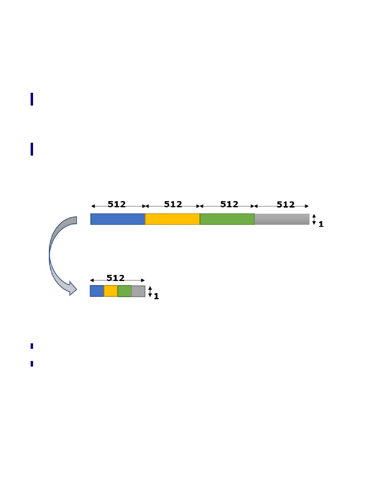
INTEL® ADVANCED MATRIX EXTENSIONS (INTEL® AMX)
The optimal size, therefore, depends very much on the DL network topology and convolution-blocking
parameters. Performance studies show that the number of iterations of M_ACC * N_ACC blocks before
proceeding to post-convolution iteration may vary from 1 to 7.
As AMX instructions generate a higher precision output (32-bit integers or 32-bit floats) from lower preci-
sion inputs (8-bit integers or 16-bit bfloats, respectively), there is a need to convert 32-bit outputs to 8-
or 16-bit inputs to be fed to the next DL network layer.
Suppose a single high-precision cache line (512-bit) is processed for conversion at a time. In that case,
there will be two or four rounds of processing until a single low-precision cache line is generated for 8- or
16-bit inputs. Potential problems include:
• the number of loads and stores of the same cache line increases 4X or 2X, respectively.
• the next round of processing of the same cache line may occur after this cache line is evicted from
DCU.
One of the optimizations mitigating these performance issues is to collect enough high-precision outputs
to convert the full low-precision cache line in a single round.
The following drawing shows the conversion flow of 32-bit integers to 8-bit integers. Each colored block
at the top represents a single full TILE output. The horizontal dimension is OFMs the vertical dimension
is spatial).
Figure 20-13. A Conversion Flow of 32-bit Integers to 8-bit Integers
To generate full 512-bit cache lines of 8-bit inputs (bottom), a multiple of 64 OFMs should be collected
before conversion. Accordingly, to generate full cache lines with 16-bit inputs, a multiple of 32 OFMs
should be collected. This often produces better performance results, though it may be viewed as a
restriction to convolution blocking parameters (in particular, N_ACC).
Example 20-19 shows the conversion code for two blocks of sixteen cache lines of 32-bit floats converted
to a single block of sixteen cache lines of 16-bit bfloats. TMUL outputs are assumed to be placed into a
scratchpad spad, and the conversion result is placed in the next_inputs buffer.
20-35

INTEL® ADVANCED MATRIX EXTENSIONS (INTEL® AMX)
Example 20-19. Two Blocks of 16 Cache Lines of 32-bit Floats Converted to One Block of 16 Cache Lines of 16-bit
BFloat
float* spad;
bfloat_16* next_inputs;
inline unsigned inputs_spatial_dim( void ) {
return /* number of pixels in map */
}
for (int i = 0; i < 16; i++)
{
__m512 f32_0 = _mm512_load_ps(spad);
__m512 f32_1 = _mm512_load_ps(spad + 16*16);
__m512 bf16 = _mm512_castsi512_ps(_mm512_cvtne2ps_pbh(f32_1, f32_0));
_mm512_store_ps(next_inputs, bf16);
spad += 16; /* Next TILE row */
next_inputs += 32 * inputs_spatial_dim();
}
Example 20-20. Using Unsigned Saturation
const int32_t db_sel[16] = { 0, 4, 8, 12, 1, 5, 9, 13, 2, 6, 10, 14, 3, 7, 11, 15 };
inline __m512i Pack_DwordsToBytes(__m512i dwords[4])
{
const __m512i sel_reg
= _mm512_load_si512(db_sel);
const __m512i words_0
= _mm512_packs_epi32(dwords[0], dwords[1]);
const __m512i words_1
= _mm512_packs_epi32(dwords[2], dwords[3]);
__m512i bytes
= _mm512_packus_epi16(words_0, words_1);
bytes
= _mm512_permutexvar_epi32(sel_reg, bytes);
return bytes;
}
20.12 INPUT AND OUTPUT BUFFERS REUSE (DOUBLE BUFFERING)
Due to the significant computational speedup achieved by the Intel AMX instructions, the performance
bottleneck of Intel AMX-enabled applications is usually memory access. The most straightforward way to
improve memory utilization is to reduce an application’s memory footprint. An application with a smaller
memory footprint will keep more of its essential data in the caches while reducing the number of costly
cache evictions. This usually improves performance.
In Deep Learning (DL), a simple, efficient way to reduce the memory footprint is to reuse the input and
output buffers of various layers in the topology.
The following simple topology illustrates where the previous layer feeds the next layer (left):
20-36
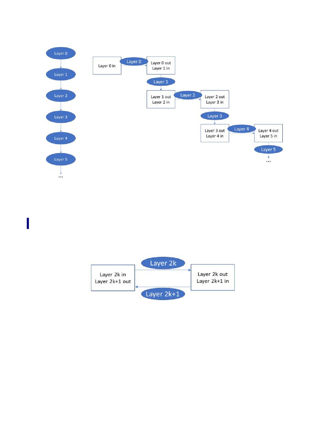
INTEL® ADVANCED MATRIX EXTENSIONS (INTEL® AMX)
Figure 20-14. Trivial Deep Learning Topology with Naive Buffer Allocation
A straightforward buffer allocation scheme is illustrated on the in Figure 20-14, in which the output of
layer N is placed into a dedicated memory buffer which is then consumed as input by layer N+1. In this
scheme, such topology with L-layers would require L+1 memory buffers, of which only the last is valuable
(containing the final results). The rest of the L memory buffers are single-use and disposable, signifi-
cantly increasing the application’s memory footprint.
The allocation scheme in Figure 20-15 offers an improved scheme whereby the entire topology only
requires two reusable memory buffers.
Figure 20-15. Minimal Memory Footprint Buffer Allocation Scheme for Trivial Deep Learning Topology
A more complex topology would require more reusable buffers, but this number is significantly smaller
than the naïve approach. ResNet-50, for example, requires only three reusable buffers (instead of 55).
Inception-ResNet-V2 requires only five reusable buffers (instead of over 250). This optimization resulted
in a 25% improved performance on the int8 end-to-end large batch throughput run of Resnet50 v1.5.
20-37

INTEL® ADVANCED MATRIX EXTENSIONS (INTEL® AMX)
20.13 SOFTWARE PREFETCHES
The CPU employs sophisticated HW prefetchers that predict future access and provide relevant data. This
works best when most memory accesses are sequential. For more details on processor hardware
prefetchers, see Section 20.13.1.2.
20.13.1 SOFTWARE PREFETCH FOR CONVOLUTION AND GEMM LAYERS
Since the Conv/GEMM kernel is centered around loops over the M, K, and N dimensions of the involved
matrices, the access will often be sequential. However, memory blocking, also recommended in this
guide, causes the CPU to re-use the same block in the A or B matrices (or both) multiple times during the
kernel execution. This means that sometimes the HW prefetcher cannot predict the subsequent access
correctly. This opens the opportunity for an SW prefetch algorithm tightly integrated into the Conv/GEMM
kernel and can bring in cache lines from future blocks based on the blocking strategy.
While the SW prefetch instruction enables selecting the target cache hierarchy level for the prefetch, this
document assumes that the prefetch will go to the MLC. The DCU is too small to prevent the prefetched
lines from being evicted before they can be used, and prefetching to LLC may not yield significant
improvement.
20.13.1.1 The Prefetch Strategy
The prefetch strategy is highly dependent on the Conv/GEMM kernel method of operation. Assuming the
“loops and blocking” design discussed earlier, the kernel operation can probably be split into multiple
phases where each phase manages a different part of the matrices (corner, middle, etc.). The developer
is encouraged to reduce the program’s size by reusing sections for repeatable matrix patterns to avoid
overflowing the instruction cache. This can be done by having each section work on relative addresses.
The SW prefetch instruction can be integrated into these sections and work on relative addresses. This
means that while one section of the code loads addresses for its use, it also prefetches memory for a
future section. The future section can be determined by looking at the future indices of any of the M/K/N
loop levels.
20.13.1.2 Prefetch Distance
One of the most important decisions when using SW prefetching is the distance between the current and
prefetched addresses. Supposing some blocking strategy is employed, it is more complex than adding an
offset to the current address. The prefetched address must be set based on the target block of the
matrix. If the target block is too close, the prefetched memory might still be in transit when the memory
is required, and the CPU will stall, waiting for it to arrive. The data might be evicted if prefetched memory
is too distant before it is used. The developer must tune the distance based on the layer/blocking param-
eters.
As an example heuristic:
• One or two loads for each TMUL operation.
• Where one matrix is already in a register.
• When two registers must be loaded.
• The recommended range between the prefetch time and the consumption time is between 100 and
500 TMUL operations.
•
100 TMUL operations should take about 1600 cycles.
• The maximum number of bytes loaded between prefetch and consumption is 1MB (500 TMUL ops /*
2 loads per ops /* 1K per tile).
• The optimum is probably closer to 100 TMUL ops. At any rate, the developer must check the current
CPU architecture and make sure that the MLC will not overflow.
20-38

INTEL® ADVANCED MATRIX EXTENSIONS (INTEL® AMX)
20.13.1.3 To Prefetch A or Prefetch B?
Whether to prefetch A, B, or both depends on the order of layer execution.
In general, the following approaches are available:
• Image affinity.
• Execute the next layer of the same image.
• Complete a single image end-to-end before continuing to the next image in the same mini-batch.
Layer affinity:
• Execute the same layer of the following image.
• Complete a layer for all images in the mini-batch before continuing to the next layer.
The activations (the result of the previous layer) in the CPU caches are seen when image affinity is used.
The weights in the caches are found when layer affinity is used. Generally, image affinity is recommended
when sizeof(A)>sizeof(B) and layer affinity otherwise. To maximize performance, the developer should
tune the switch point between the two methods. The choice between these two methods is also affected
by the target matrix for prefetching. If the developer is confident that one of the matrices will already be
present in the cache when the Conv/GEMM kernel begins execution, the potential benefit of SW
prefetching decreases dramatically.
The size of the A-matrix, B-matrix, and cache.
The developer should sum up the memory requirements of the Conv/GEMM kernel for the current layer
and compare it to the size of the cache (MLC). Combined with the previous step, it can indicate whether
SW prefetching can yield any performance benefit. When large matrices are involved, there is a greater
chance for improvement when prefetching the A- and the B-matrices.
20.13.1.4 To Prefetch or Not to Prefetch C?
It is not the C-matrix we might want to prefetch but rather the final output matrix of the layer, after its
post-convolution or post-GEMM phase, including quantization to a lower precision data type. Generally,
prefetch those cache lines ahead of time since, with double buffering, these might have been read by
previous layers, possibly executed in other cores.
Use the PREFETCHW instruction to read those cache lines into the DCU just in time for the store opera-
tions to find them in the DCU ready to be written, avoiding Read For Ownership latency that otherwise
delays store completion. The exact timing of issuing the PREFETCHW instruction depends on multiple
factors and requires careful tuning to get it right.
20.13.2 SOFTWARE PREFETCH FOR EMBEDDING LAYER
When the memory access pattern is semi-random, it is often impossible for the HW prefetcher to predict
since it is based on application logic. In this case, the application may benefit from “proactive”
prefetching using the SW prefetch instructions of addresses the application knows it will access soon.
An excellent example is Deep Learning, wherein the recommendation systems often use the embedding
layer. The core loop of the embedding algorithm loads indices from an index buffer, and for each index, it
loads the corresponding row from the embedding table for further processing. While the index buffer may
contain duplicate indices that benefit from CPU caching, the pattern is often considered random or semi-
random. This can make the HW prefetcher less efficient. Since the entire content of the index buffer is
already known, rows soon to be encountered can be prefetched to the DCU.
20-39

INTEL® ADVANCED MATRIX EXTENSIONS (INTEL® AMX)
Example 20-21. Prefetching Rows to the DCU
1
void prefetched_embedding(uint32_t *a, float *e, float *c, size_t num_indices,
2
float scale, float bias, size_t lookahead)
3
{
4
__m512 s = _mm512_set1_ps(scale);
5
__m512 b = _mm512_set1_ps(bias);
6
7
for (size_t i = 0; i < num_indices; i++) {
8
_mm_prefetch(
9
(char const *)&e[a[i + lookahead] * FLOATS_PER_CACHE_LINE],
10
_MM_HINT_T0);
11
__m512 ereg =
12
_mm512_load_ps(&e[((size_t)a[i]) * FLOATS_PER_CACHE_LINE]);
13
__m512 creg = _mm512_fmadd_ps(ereg, s, b);
14
_mm512_store_ps(&c[i * FLOATS_PER_CACHE_LINE], creg);
15
}
16
}
20.14 STORE TO LOAD FORWARDING
Before it gets written to the DCU (first-level cache), store instructions copy data from general purpose,
vector, or tile registers into store buffers. All load instructions, other than TileLoad, can load the data they
are looking for from the store buffers and memory hierarchy.
The TileLoad instruction can’t load data from store buffers. It can only detect that the data is there and
must wait until it is written to the memory hierarchy. Once written, TileLoad can read it from the memory
hierarchy. This incurs a significant slowdown.
TileStore forwarding to non-TileLoad instructions via store buffers is supported under one restriction:
they must both be of cache line size (64 bytes).
Forwarding is generally not advised because this mechanism has outliers. To avoid store-to-load
forwarding, ensure enough distance between those two operations in the order of 10s of cycles in time.
20.15 MATRIX TRANSPOSE
This section describes the best-known SW implementations for several matrix transformations of BF16
data.
In this context, flat format means:
• Normal (i.e., non-VNNI).
• Unblocked rows (rows of matrices occupy a consecutive region in memory).
The first condition is essential. The second could be relaxed by changing the code in Example 20-22
accordingly. VNNI format implies only the second condition (non-blocking of rows). It is important to
note that the MxN matrix in flat format will be represented by a (M/2)x(N/*2) matrix in VNNI format.
20-40

INTEL® ADVANCED MATRIX EXTENSIONS (INTEL® AMX)
20.15.1 FLAT-TO-FLAT TRANSPOSE OF BF16 DATA
The primitive block transposed in this algorithm is 32x8 (i.e., 32 rows, eight BF16 numbers each), which
is transformed into an 8x32 block (i.e., eight rows of 32 BF16 numbers each).
The implementation uses sixteen ZMM registers and three mask registers.
Input parameters: MxN, sizes of the rectangular block to be transposed. Assuming M is a multiple of 32,
and N is a multiple of eight, we may also assume in Example 20-22:
• I_STRIDE is the row size of the input matrix in bytes.
• O_STRIDE is the row size of the output buffer in bytes.
• r8 contains starting address of the input matrix.
• r9 contains starting address of the output buffer.
Example 20-22. BF16 Matrix Transpose (32x8 to 8x32)
/*1 of 2 */
1
mov
r10,
0xf0
2
kmovd
k1,
r10d
3
mov
r10,
0xf00
4
kmovd
k2,
r10d
5
mov
r10,
0xf000
6
kmovd
k3,
r10d
7
mov
rax,
N / 8
L.N:
8
mov
rdx,
M / 32
L.M:
9
vbroadcasti32x4 zmm0,
xmmword ptr [r8]
10
vbroadcasti32x4 zmm0{k1},
xmmword ptr [r8+I_STRIDE*8]
11
vbroadcasti32x4 zmm0{k2},
xmmword ptr [r8+I_STRIDE*16]
12
vbroadcasti32x4 zmm0{k3},
xmmword ptr [r8+I_STRIDE*24]
13
vbroadcasti32x4 zmm1,
xmmword ptr [r8+I_STRIDE*1]
14
vbroadcasti32x4 zmm1{k1},
xmmword ptr [r8+I_STRIDE*9]
15
vbroadcasti32x4 zmm1{k2},
xmmword ptr [r8+I_STRIDE*17]
16
vbroadcasti32x4 zmm1{k3},
xmmword ptr [r8+I_STRIDE*25]
17
vbroadcasti32x4 zmm2,
xmmword ptr [r8+I_STRIDE*2]
18
vbroadcasti32x4 zmm2{k1},
xmmword ptr [r8+I_STRIDE*10]
19
vbroadcasti32x4 zmm2{k2},
xmmword ptr [r8+I_STRIDE*18]
20
vbroadcasti32x4 zmm2{k3},
xmmword ptr [r8+I_STRIDE*26]
21
vbroadcasti32x4 zmm3,
xmmword ptr [r8+I_STRIDE*3]
22
vbroadcasti32x4 zmm3{k1},
xmmword ptr [r8+I_STRIDE*11]
23
vbroadcasti32x4 zmm3{k2},
xmmword ptr [r8+I_STRIDE*19]
24
vbroadcasti32x4 zmm3{k3},
xmmword ptr [r8+I_STRIDE*27]
25
vbroadcasti32x4 zmm4,
xmmword ptr [r8+I_STRIDE*4]
26
vbroadcasti32x4 zmm4{k1},
xmmword ptr [r8+I_STRIDE*12]
27
vbroadcasti32x4 zmm4{k2},
xmmword ptr [r8+I_STRIDE*20]
28
vbroadcasti32x4 zmm4{k3},
xmmword ptr [r8+I_STRIDE*28]
29
vbroadcasti32x4 zmm5,
xmmword ptr [r8+I_STRIDE*5]
30
vbroadcasti32x4 zmm5{k1},
xmmword ptr [r8+I_STRIDE*13]
31
vbroadcasti32x4 zmm5{k2},
xmmword ptr [r8+I_STRIDE*21]
32
vbroadcasti32x4 zmm5{k3},
xmmword ptr [r8+I_STRIDE*29]
33
vbroadcasti32x4 zmm6,
xmmword ptr [r8+I_STRIDE*6]
20-41

INTEL® ADVANCED MATRIX EXTENSIONS (INTEL® AMX)
/*2 of 2 */
34
vbroadcasti32x4 zmm6{k1},
xmmword ptr [r8+I_STRIDE*14]
35
vbroadcasti32x4 zmm6{k2},
xmmword ptr [r8+I_STRIDE*22]
36
vbroadcasti32x4 zmm6{k3},
xmmword ptr [r8+I_STRIDE*30]
37
vbroadcasti32x4 zmm7,
xmmword ptr [r8+I_STRIDE*7]
38
vbroadcasti32x4 zmm7{k1},
xmmword ptr [r8+I_STRIDE*15]
39
vbroadcasti32x4 zmm7{k2},
xmmword ptr [r8+I_STRIDE*23]
40
vbroadcasti32x4 zmm7{k3},
xmmword ptr [r8+I_STRIDE*31]
41
vpunpcklwd
zmm8,
zmm0,
zmm1
42
vpunpckhwd
zmm9,
zmm0,
zmm1
43
vpunpcklwd
zmm10,
zmm2,
zmm3
44
vpunpckhwd
zmm11,
zmm2,
zmm3
45
vpunpcklwd
zmm12,
zmm4,
zmm5
46
vpunpckhwd
zmm13,
zmm4,
zmm5
47
vpunpcklwd
zmm14,
zmm6,
zmm7
48
vpunpckhwd
zmm15,
zmm6,
zmm7
49
vpunpckldq
zmm0,
zmm8,
zmm10
50
vpunpckhdq
zmm1,
zmm8,
zmm10
51
vpunpckldq
zmm2,
zmm9,
zmm11
52
vpunpckhdq
zmm3,
zmm9,
zmm11
53
vpunpckldq
zmm4,
zmm12,
zmm14
54
vpunpckhdq
zmm5,
zmm12,
zmm14
55
vpunpckldq
zmm6,
zmm13,
zmm15
56
vpunpckhdq
zmm7,
zmm13,
zmm15
57
vpunpcklqdq
zmm8,
zmm0,
zmm4
58
vpunpckhqdq
zmm9,
zmm0,
zmm4
59
vpunpcklqdq
zmm10,
zmm1,
zmm5
60
vpunpckhqdq
zmm11,
zmm1,
zmm5
61
vpunpcklqdq
zmm12,
zmm2,
zmm6
62
vpunpckhqdq
zmm13,
zmm2,
zmm6
63
vpunpcklqdq
zmm14,
zmm3,
zmm7
64
vpunpckhqdq
zmm15,
zmm3,
zmm7
65
vmovdqu16
zmmword ptr [r9],
zmm8
66
vmovdqu16
zmmword ptr [r9+O_STRIDE],
zmm9
67
vmovdqu16
zmmword ptr [r9+O_STRIDE*2],
zmm10
68
vmovdqu16
zmmword ptr [r9+O_STRIDE*3],
zmm11
69
vmovdqu16
zmmword ptr [r9+O_STRIDE*4],
zmm12
70
vmovdqu16
zmmword ptr [r9+O_STRIDE*5],
zmm13
71
vmovdqu16
zmmword ptr [r9+O_STRIDE*6],
zmm14
72
vmovdqu16
zmmword ptr [r9+O_STRIDE*7],
zmm15
73
add
r9, 0x40
74
add
r8, I_STRIDE*32
75
dec
rdx
76
jnz
L.M
77
add
r9, (O_STRIDE*8 — (M/32) * 0X40)
78
sub
r8, (I_STRIDE*M-0x10)
79
dec
rax
80
jnz
L.N
20-42
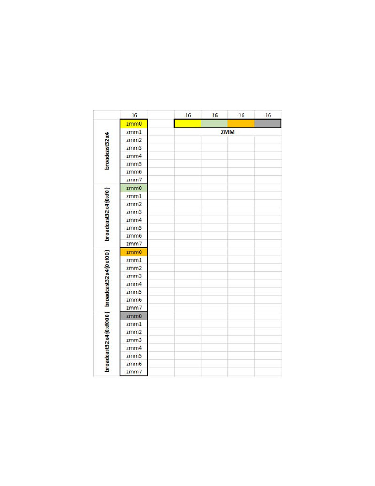
INTEL® ADVANCED MATRIX EXTENSIONS (INTEL® AMX)
Implementation discussion:
• Lines 1-6 set mask registers k1, k2, k3.
• Lines 7 and 8 put trip counts for primitive blocks in N- and M-dimensions, respectively.
• Lines 9-72 implement the transpose of a primitive block 32x8. It uses 16 ZMM registers (zmm0-
zmm15).
• Lines 9-40 implement loading 32 quarter-cache lines into 8 ZMM registers, according to the following
picture (numbers are in bytes):
Figure 20-16. Loading 32 Quarter-Cache Lines into 8 ZMM Registers
• Lines 41-64 are transpose flow proper. It creates a transposed block 8x32 in registers zmm8-zmm15.
• Lines 65-72 store transposed block 8x32 to the output buffer.
20-43

INTEL® ADVANCED MATRIX EXTENSIONS (INTEL® AMX)
20.15.2 VNNI-TO-VNNI TRANSPOSE
The primitive block transposed in this algorithm is 8x8 (i.e., eight rows, eight BF16 numbers each), which
is transformed into a2x32 block (i.e., two rows of 32 BF16 numbers each).
The implementation uses five ZMM registers and three mask registers.
Input parameters:
• MxN, sizes of the rectangular block to be transposed (in VNNI format); it is assumed that M, N are
multiples of eight.
• I_STRIDE is the row size of the input matrix in bytes.
• O_STRIDE is the row size of the output buffer in bytes.
• r8 contains starting address to the input matrix.
• r9 contains starting address to the output buffer.
• zmm31 is preloading with four copies of the following constant: unsigned int shuflle_cntrl[4] =
{0x05040100, 0x07060302, 0x0d0c0908, 0x0f0e0b0a};
Example 20-23. BF16 VNNI-to-VNNI Transpose (8x8 to 2x32)
1
mov r10, 0xf0
2
kmovd k1, r10d
3
mov r10, 0xf00
4
kmovd k2, r10d
5
mov r10, 0xf000
6
kmovd k3, r10d
7
mov rax, N / 8
L.N:
8 mov rdx, M / 8
L.M:
9 vbroadcasti32x4 zmm0, xmmword ptr [r8]
10 vbroadcasti32x4 zmm0{k1}, xmmword ptr [r8+I_STRIDE*2]
11 vbroadcasti32x4 zmm0{k2}, xmmword ptr [r8+I_STRIDE*4]
12 vbroadcasti32x4 zmm0{k3}, xmmword ptr [r8+I_STRIDE*6]
13 vbroadcasti32x4 zmm1, xmmword ptr [r8+I_STRIDE*1]
14 vbroadcasti32x4 zmm1{k1}, xmmword ptr [r8+I_STRIDE*3]
15 vbroadcasti32x4 zmm1{k2}, xmmword ptr [r8+I_STRIDE*5]
16 vbroadcasti32x4 zmm1{k3}, xmmword ptr [r8+I_STRIDE*7]
17 vpshufb zmm2, zmm0, zmm31
18 vpshufb zmm3, zmm1, zmm31
19 vpunpcklqdq zmm0, zmm2, zmm3
20 vpunpckhqdq zmm1, zmm2, zmm3
21 vmovdqu16 zmmword ptr [r9], zmm0
22 vmovdqu16 zmmword ptr [r9+O_STRIDE], zmm1
23 add r9, 0x40
24 add r8, I_STRIDE*8
25 dec rdx
26 jnz L.M
27 add r9, (O_STRIDE*2 - (M/8) * 0x40)
28 sub r8, (I_STRIDE*M-0x10)
29 dec rax
30 jnz L.N
20-44
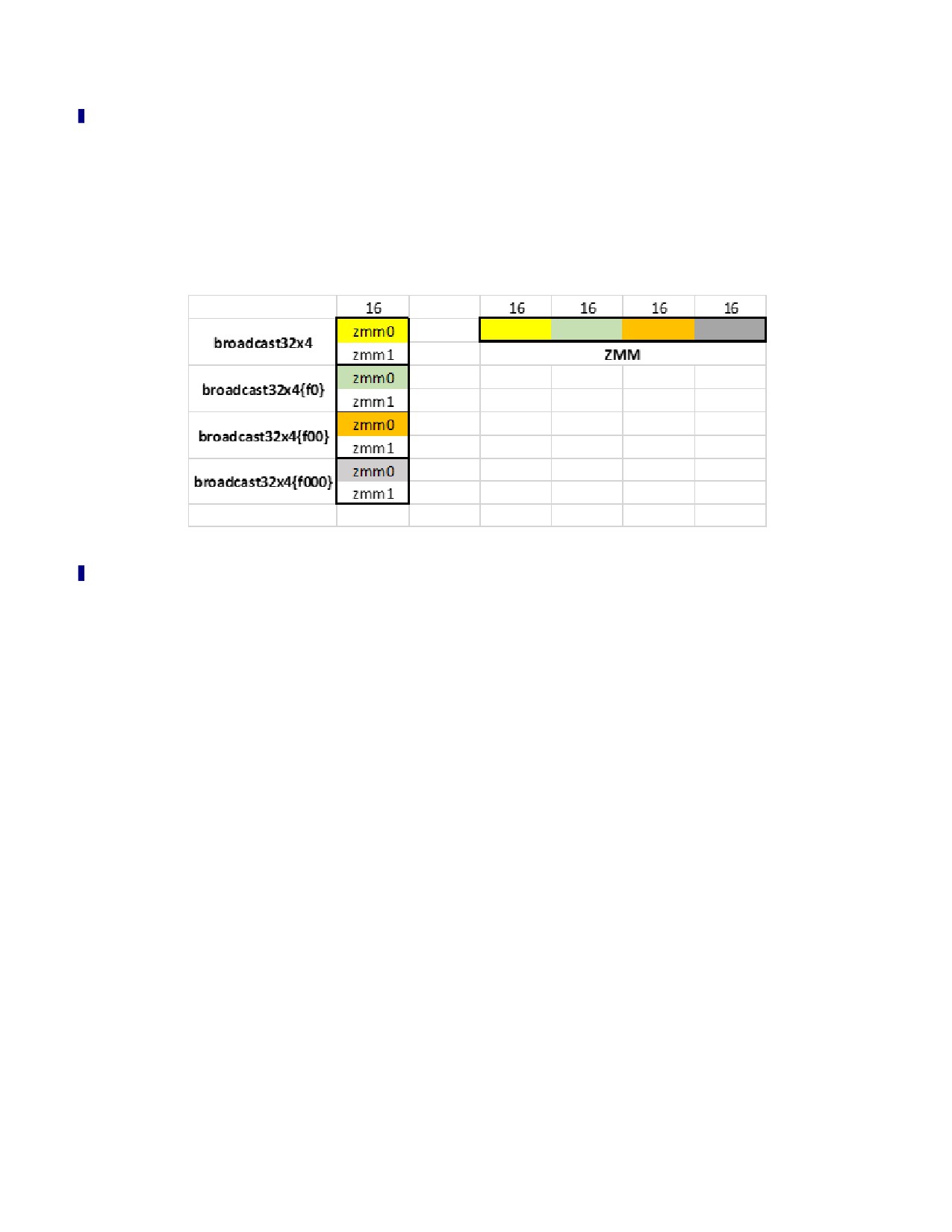
INTEL® ADVANCED MATRIX EXTENSIONS (INTEL® AMX)
BF16 VNNI-to-VNNI Transpose Implementation Discussion
• Lines 1-6 set mask registers k1, k2, k3.
• Lines 7 and 8 put trip counts for primitive blocks in N- and M-dimensions, respectively.
• Lines 9-22 implement the transpose of a primitive block 32x8. It uses five ZMM registers (zmm0-
zmm3, zmm31).
• Lines 9-16 implement loading eight quarter-cache lines into two ZMM registers, according to
Figure 20-17 (numbers are in bytes):
Figure 20-17. Loading Eight Quarter-Cache Lines into Two ZMM Registers
• Lines 17-20 implement simultaneous transpose of four 2x2 blocks of QWORDs (i.e., 2x8 blocks of
BF16). It creates a transposed block 2x32 in registers zmm2-zmm3.
• Lines 21-22 store transposed block 2x32 to the output buffer.
20-45
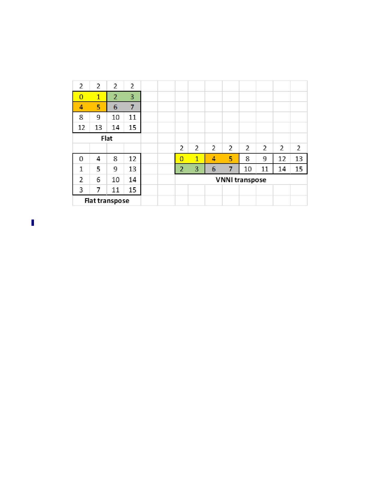
INTEL® ADVANCED MATRIX EXTENSIONS (INTEL® AMX)
20.15.3 FLAT-TO-VNNI TRANSPOSE
The algorithm below is based on: Flat-to-VNNI transpose of WORDs is equivalent to Flat-to-Flat trans-
pose of DWORDs. This is illustrated below (the header numbers are bytes):
Figure 20-18. Flat-to-VNNI Transpose of WORDs Equivalence to Flat-to-Flat Transpose of DWORDs
The primitive block transposed in this algorithm is 16x8 (i.e., 16 rows, 8 BF16 numbers each), which is
transformed into a 4x32 block (i.e., four rows of 32 BF16 numbers each).
The implementation uses eight ZMM registers and three mask registers.
Input parameters:
• MxN, sizes of the rectangular block to be transposed; it is assumed that M multiple of 16, N multiple
of eight.
• I_STRIDE is the row size of the input matrix in bytes.
• O_STRIDE is the row size of the output buffer in bytes.
• r8 contains the starting address for the input matrix.
• r9 contains the starting address for the output buffer.
20-46

INTEL® ADVANCED MATRIX EXTENSIONS (INTEL® AMX)
Example 20-24. BF16 Flat-to-VNNI Transpose (16x8 to 4x32)
1
mov r10, 0xf0
2
kmovd k1, r10d
3
mov r10, 0xf00
4
kmovd k2, r10d
5
mov r10, 0xf000
6
kmovd k3, r10d
7
mov rax, N / 8
L.N:
8
mov rdx, M / 16
L.M:
9
vbroadcasti32x4 zmm0, xmmword ptr [r8]
10
vbroadcasti32x4 zmm0{k1}, xmmword ptr [r8+I_STRIDE*4]
11
vbroadcasti32x4 zmm0{k2}, xmmword ptr [r8+I_STRIDE*8]
12
vbroadcasti32x4 zmm0{k3}, xmmword ptr [r8+I_STRIDE*12]
13
vbroadcasti32x4 zmm1, xmmword ptr [r8+I_STRIDE*1]
14
vbroadcasti32x4 zmm1{k1}, xmmword ptr [r8+I_STRIDE*5]
15
vbroadcasti32x4 zmm1{k2}, xmmword ptr [r8+I_STRIDE*9]
16
vbroadcasti32x4 zmm1{k3}, xmmword ptr [r8+I_STRIDE*13]
17
vbroadcasti32x4 zmm2, xmmword ptr [r8+I_STRIDE*2]
18
vbroadcasti32x4 zmm2{k1}, xmmword ptr [r8+I_STRIDE*6]
19
vbroadcasti32x4 zmm2{k2}, xmmword ptr [r8+I_STRIDE*10]
20
vbroadcasti32x4 zmm2{k3}, xmmword ptr [r8+I_STRIDE*14]
21
vbroadcasti32x4 zmm3, xmmword ptr [r8+I_STRIDE*3]
22
vbroadcasti32x4 zmm3{k1}, xmmword ptr [r8+I_STRIDE*7]
23
vbroadcasti32x4 zmm3{k2}, xmmword ptr [r8+ I_STRIDE*11]
24
vbroadcasti32x4 zmm3{k3}, xmmword ptr [r8+ I_STRIDE*15]
25
vpunpckldq zmm4, zmm0, zmm1
26
vpunpckhdq zmm5, zmm0, zmm1
27
vpunpckldq zmm6, zmm2, zmm3
28
vpunpckhdq zmm7, zmm2, zmm3
29
vpunpcklqdq zmm0, zmm4, zmm6
30
vpunpckhqdq zmm1, zmm4, zmm6
31
vpunpcklqdq zmm2, zmm5, zmm7
32
vpunpckhqdq zmm3, zmm5, zmm7
33
vmovups zmmword ptr [r9], zmm0
34
vmovups zmmword ptr [r9+O_STRIDE], zmm1
35
vmovups zmmword ptr [r9+O_STRIDE*2], zmm2
36
vmovups zmmword ptr [r9+O_STRIDE*3], zmm3
37
add r9, 0x40
38
add r8, I_STRIDE*16
39
dec rdx
40
jnz L.M
41
add r9, (O_STRIDE*4 - (M/16)*0x40)
42
sub r8, (I_STRIDE*M-0x10)
43
dec rax
44
jnz L.N
20-47
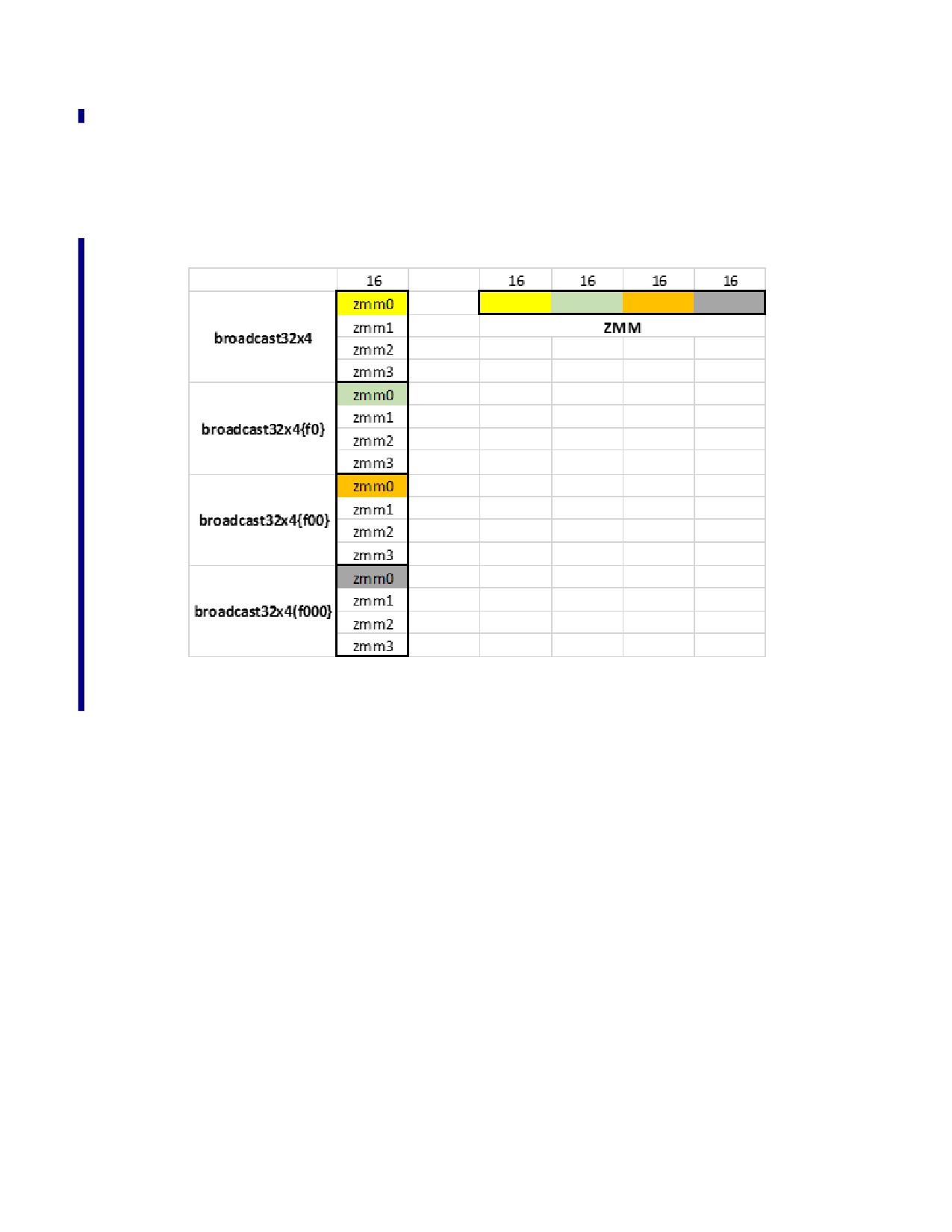
INTEL® ADVANCED MATRIX EXTENSIONS (INTEL® AMX)
Implementation Discussion
• Lines 1-6 set mask registers k1, k2, k3.
• Lines 7 and 8 put trip counts for primitive blocks in N- and M-dimensions, respectively.
• Lines 9-36 implement the transpose of a primitive block 16x8. It uses eight ZMM registers (zmm0-
zmm7).
• Lines 9-24 implement loading 16 quarter-cache lines into four ZMM registers zmm0-zmm3,
according to Figure 20-19 (numbers are in bytes):
Figure 20-19. BF16 Flat-to-VNNI Transpose
• Lines 25-32 are the transpose flow proper. It creates a transposed block 4x32 in registers zmm0-
zmm3.
• Lines 33-36 store transposed block 4x32 to the output buffer.
20.15.4 FLAT-TO-VNNI RE-LAYOUT
The primitive block which is being re-layout in this algorithm is 2x32 (i.e., 2 rows, 32 BF16 numbers
each), which is transformed into a 1x64 block (i.e., 1 rows of 64 BF16 numbers each).
The implementation uses 5 ZMM registers and no mask registers.
Input parameters:
• MxN, sizes of the rectangular block to be transposed; it is assumed that M multiple of 2, N multiple
of 32.
• I_STRIDE is the row size of input matrix in bytes.
• O_STRIDE is the row size of output buffer in bytes.
• r8 contains starting address to input matrix.
• r9 contains starting address to output buffer.
• zmm30, zmm31 are preloaded with following constants, respectively:
20-48

INTEL® ADVANCED MATRIX EXTENSIONS (INTEL® AMX)
• const short perm_cntl_1[32] = {0x00, 0x20, 0x01, 0x21, 0x02, 0x22, 0x03, 0x23, 0x04, 0x24,
0x05, 0x25, 0x06, 0x26, 0x07, 0x27, 0x08, 0x28, 0x09, 0x29, 0x0a, 0x2a, 0x0b, 0x2b, 0x0c, 0x2c,
0x0d, 0x2d, 0x0e, 0x2e, 0x0f, 0x2f};
• const short perm_cntl_2[32] = {0x30, 0x10, 0x31, 0x11, 0x32, 0x12, 0x33, 0x13, 0x34, 0x14,
0x35, 0x15, 0x36, 0x16, 0x37, 0x17, 0x38, 0x18, 0x39, 0x19, 0x3a, 0x1a, 0x3b, 0x1b, 0x3c, 0x1c,
0x3d, 0x1d, 0x3e, 0x1e, 0x3f, 0x1f};
Example 20-25. BF16 Flat-to-VNNI Re-Layout
1
mov rdx, M / 2
L.M:
2
mov rax, N / 32
L.N:
3
vmovups zmm0, zmmword ptr [r8]
4
vmovups zmm1, zmmword ptr [r8+I_STRIDE]
5
vmovups zmm2, zmm0
6
vpermt2w zmm2, zmm30, zmm1
7
vpermt2w zmm1, zmm31, zmm0
8
vmovups zmmword ptr [r9], zmm2
9
vmovups zmmword ptr [r9+0x40], zmm1
10
add r9, 0x80
11
add r8, 0x40
12
dec rax
13
jnz L.N
14
add r9, (O_STRIDE - (N/32)*0x80)
15
add r8, (I_STRIDE*2 - (N/32)*0x40)
16
dec rdx
17
jnz L.M
BF16 Flat-to-VNNI Re-Layout Implementation Discussion
• Lines 1, 2 put trip counts for primitive blocks in N- and M-dimensions, respectively.
• Lines 3, 4 implement loading two full cache lines into two ZMM registers zmm0-zmm1, from
consecutive rows of the input matrix.
• Lines 5 through 7 implement the re-layout of a primitive block 2x32. It uses five ZMM registers
(zmm0-zmm2, zmm30-zmm31).
• Lines 8, 9 implement storing two full cache lines in two ZMM registers zmm1-zmm2, into consecutive
columns of the output matrix.
20-49

INTEL® ADVANCED MATRIX EXTENSIONS (INTEL® AMX)
20.16 MULTI-THREADING CONSIDERATIONS
20.16.1 THREAD AFFINITY
As with Intel AVX-512 code, it is advised to fully define thread affinity and object affinity to process a
single object in the same physical core, thus keeping the activations in core caches (unless larger than
the size of the caches). This advice becomes imperative with Intel AMX code since those applications are
more sensitive to memory-related issues.
20.16.2 INTEL® HYPER-THREADING TECHNOLOGY (INTEL® HT)
Running more than one Intel AMX thread on the same physical core may result in overall performance
loss due to the two threads competing for the same hardware resources. Scheduling a non-Intel AMX
thread next to an Intel AMX thread on the same core may decrease the thread performance more than
one expects due to normal competition for resources.
For optimum performance, please choose one of the following options in priority order:
1. Schedule one Intel AMX thread per physical core on one of its logical processors, while leaving the
other logical processors idle.
2. Affintize a software thread that executes an endless TPAUSE CO.2 loop next to the Intel AMX thread.
a. This prevents other threads from being scheduled on that logical processor.
1) All hardware resources within the physical core are therefore allocated to the Intel AMX
thread.
2) This endless loop thread must terminate when the Intel AMX thread is about to terminate.
3. Code pause loops of thread pool threads that are waiting for the next task to be assigned to them
with UMWAIT or TPAUSE C0.2 rather than with PAUSE, TPAUSE C0.1, or a non-pausing spin.
20.16.3 WORK PARTITIONING BETWEEN CORES
Deep Learning (DL) applications must often adhere to latency requirements that cannot be fulfilled within
a single core. In these cases, a single object’s processing must be partitioned between multiple cores.
Additionally, often the output of one layer is the input of the next layer. Due to the nature of the compu-
tations in DL applications, partitioning over different dimensions (N, M, K) will have different implications
for the data locality in the core’s caches. Minimize importing data from a different core’s caches if possible
as this can hamper performance.
20-50
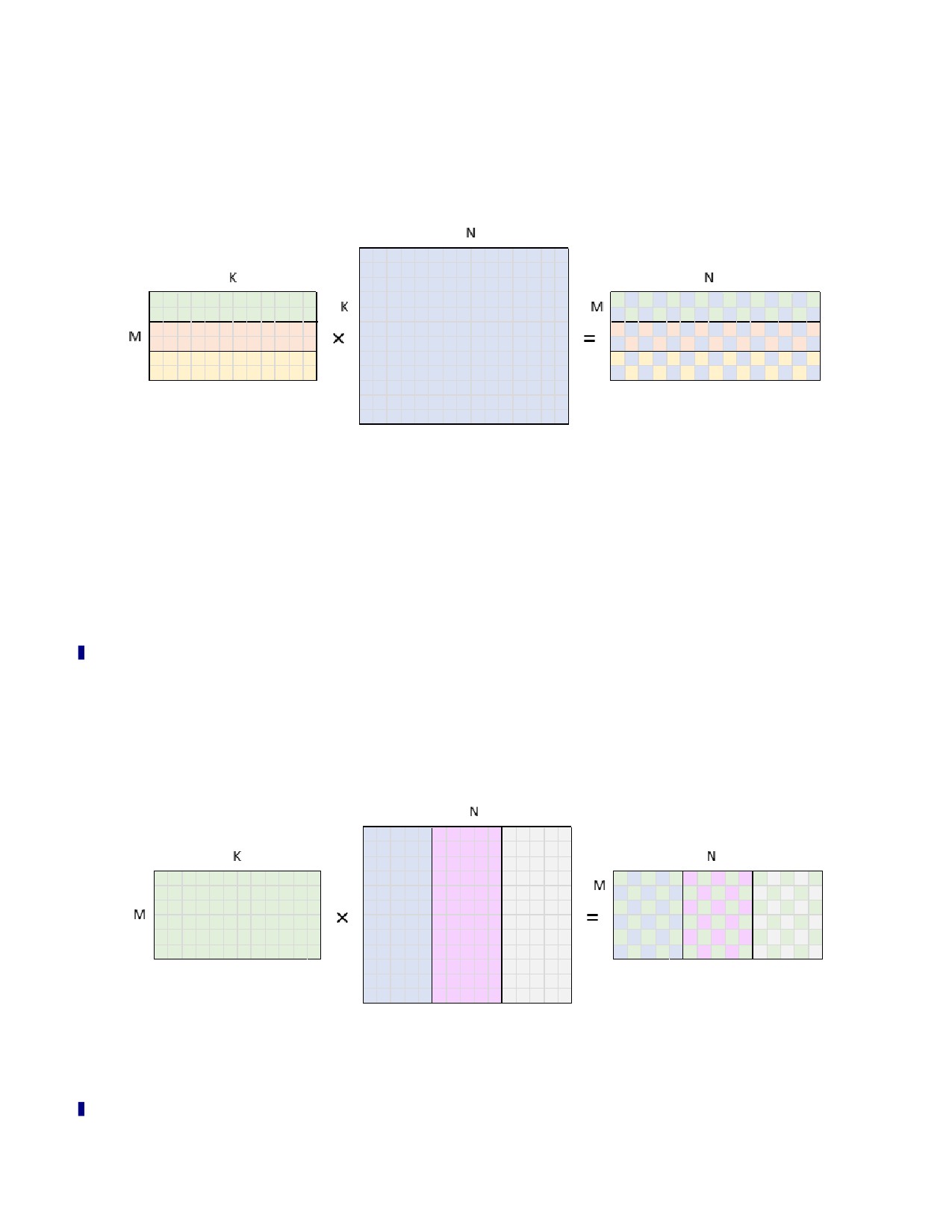
INTEL® ADVANCED MATRIX EXTENSIONS (INTEL® AMX)
20.16.3.1 Partitioning Over M
Partitioning a DL layer over the M dimension has the advantage of nearly complete data locality. The
layer’s output is also partitioned by M between the cores and is, therefore, already in the cache of the
corresponding core at the beginning of the next layer. Figure 20-20 shows this schematically.
Figure 20-20. GEMM Data Partitioning Between Three Cores in a Layer Partitioned by the M-Dimension
Here the data read and written by each of the three cores is bound by a black rectangle.
It should be noted that in the case of convolutions, limited overlap in the M-dimension of the activations
occurs between neighboring cores. Due to the convolutions, a finite-sized filter is slid over the activa-
tions. Thus, the M-dimension overlaps (KH-1)/*W (refer to Example 20-13) between the two neighboring
cores.
• Advantages: When multiple layers in a chain are partitioned by the M-dimension between the same
number of cores, each core has its data in its local cache.
• Disadvantages: All the cores read the B-matrix (or weights in convolutions) entirely, which might
pose a bandwidth problem if the B-matrix is large.
20.16.3.2 Partitioning Over N
Partitioning a DL layer over the N-dimension reduces the read bandwidth in GEMMs with large B-matrices
or large weights in convolutions. Each core reads a portion of the B-matrix in this scenario:
Figure 20-21. GEMM Data Partitioning Between Three Cores in a Layer Partitioned by the N-Dimension
Unfortunately, the output of the layer is also partitioned by the N-dimension between the cores, which is
incompatible with M and N partitioning of the subsequent layer. For visualization, compare the right side
20-51
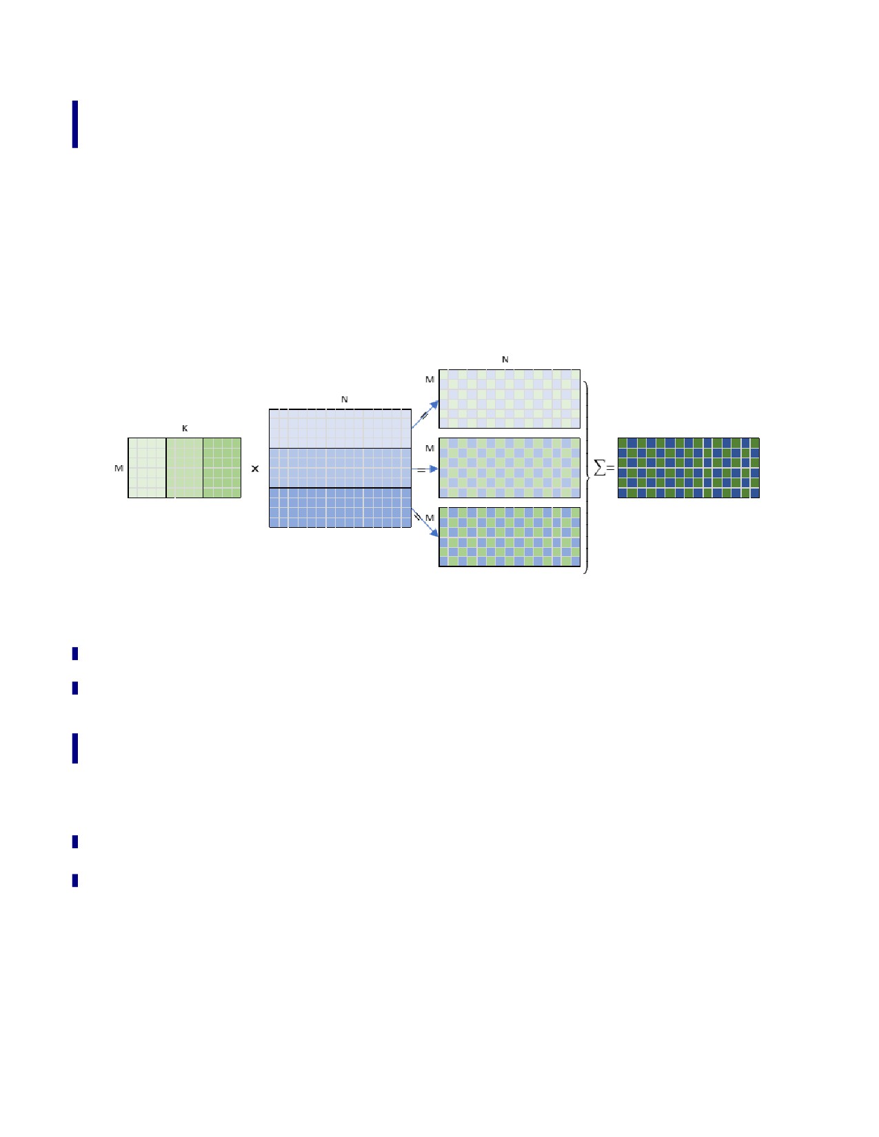
INTEL® ADVANCED MATRIX EXTENSIONS (INTEL® AMX)
of Figure 20-21 to the left side of Figures 20-20 and 20-21. In this scenario, a core in the subsequent
layer is guaranteed to have most of its data from outside its local caches. This is not the case in K-dimen-
sion partitioning (see Section 20.16.3.3), but it also comes at a price.
• Advantages: It may reduce read bandwidth significantly in case of large B / large weights.
• Disadvantages: If the next layer is partitioned by M or by N, most of the activations in the next layer
will not reside in the local caches of the corresponding cores.
20.16.3.3 Partitioning Over K
Partitioning a DL layer over the K-dimension reduces the read bandwidth in GEMMs with large K-dimen-
sions by reducing the amount of data being read from the A- and B-matrices (activations and weights in
convolutions). Each core reads a portion of the matrices in this scenario, as illustrated in Figure 20-22.
Figure 20-22. GEMM Data Partitioning Between Three Cores in a Layer Partitioned by the K-Dimension
Additionally, if a layer is partitioned by the N-dimension and the subsequent layer is partitioned by the K-
dimension, the activation data will reside in the local caches of the cores in layer partitioned by the K-
dimension. For visualization, compare the right side of Figure 20-21 with the left side of Figure 20-22.
Unfortunately, this comes at a price: each core prepares partial results of the entire C-matrix. To obtain
final results, either a mutex (or several mutexes) is required to guard the write operations into the C-
matrix, or a reduction operation is needed at the end of the layer. The mutex solution is not advised
because threads will be blocked for a significant time. A reduction runs the risk of being costly since it
entails the following:
• A synchronization barrier is required before the reduction.
• Reading a potentially large amount of data during the reduction:
— There are T copies of the C-matrix, where T is the number of threads (the example has three).
— The size of the matrices before the reduction is x2 (in case of a bfloat16 datatype) or x4 (in case
of int8 datatype) times larger than the output C-matrix.
— During the reduction, most of the cores’ data will come outside their local cache hierarchy.
20-52

INTEL® ADVANCED MATRIX EXTENSIONS (INTEL® AMX)
20.16.3.4 Memory Bandwidth Implications of Work Partitioning Over Multiple Dimensions
OpenMP offers a convenient interface for nested loop parallelization. For example, one could partition the
N, M, and K dimensions can be partitioned automatically between threads using Example 20-26.
Example 20-26. GEMM Parallelized with omp Parallel for Collapse
#pragma omp parallel for collapse(2)
for (int n = 0; n < N; n += N_ACC*TILE_N) {
for (int m = 0; m < M; m += M_ACC*TILE_M) {
}
}
The collapse clause specifies how many loops within a nested loop should be collapsed into a single iter-
ation space and divided between the threads. The order of the iterations in the collapsed iteration space
is the same as though they were executed sequentially.
If there is no specified schedule, OpenMP automatically uses schedule(static,1), resulting in the sequen-
tial assignment of loop iterations to threads.
If we assume N=4*N_ACC*TILE_N and M=4*M_ACC*TILE_M wherein the K-dimension is deliberately excluded
from consideration due to its problematic nature, there would be 4*4=16 iterations in the two nested
loops. Now assume the division of iterations between three threads. As shown in Table 20-7, the code in
Example 20-26 would result in a partition of the iterations between threads.
Table 20-7. A Simple Partition of Work Between Three Threads
A
B
C
Thread 0:
0.0
0.3
1.2
2.1
3.0
3.3
100%
100%
38%
Thread 1:
0.1
1.0
1.3
2.2
3.1
100%
100%
100%
Thread 2:
0.2
1.1
2.0
2.3
3.2
100%
100%
100%
Where every cell of the form n’,m’ contains the n’=n/N_ACC*TILE_N and m’=m/M_ACC*TILE_M indices
from the loops in Example 20-19.
It is clear from Table 20-7 that each of the three threads executes at least one iteration with n’=0,1,2,3
and at least one iteration with m’=0,1,2,3. This means that every thread reads all of A and all of B.
By rearranging the work between threads in the following partitioning, the size of the B read is reduced
by each thread by 50%, which might be significant in workloads where B is large. Similarly, the size of A
can be reduced by 50% by swapping m’ and n’ indices for workloads with a large A.
Table 20-8. An Optimized Partition of Work Between Three Threads
A
B
C
Thread 0:
0.0
0.1
0.2
0.3
3.0
3.1
100%
50%
38%
Thread 1:
1.0
1.1
1.2
1.3
3.2
3.3
100%
50%
38%
Thread 2:
2.0
2.1
2.2
2.3
100%
25%
25%
20-53

INTEL® ADVANCED MATRIX EXTENSIONS (INTEL® AMX)
20.16.4 RECOMMENDATION SYSTEM EXAMPLE
Many recommendation systems are built from a few GEMM layers that follow each other, an Embedding
layer, and a layer connecting them. They are generally split into four distinct tasks:
1. Bottom GEMMs (MLPs).
2. Embedding.
3. Bottom MLP + Embedding Concat, GEMM, and Reshape.
4. Top GEMMs (MLPs).
The first two are independent so that they can execute in parallel. Their output feeds into the third task,
whose output, in turn, feeds into the fourth task.
A few notes:
• Recommendation systems usually use a large batch to rank a reasonably large set of options.
• The GEMM layers are usually compute- or cache-bandwidth limited, whereas the Embedding layer is
memory-bandwidth limited.
• Recommendation systems are real-time and therefore limited to a specific latency.
When the latency requirement is a few milliseconds, the recommendation system topology has to be
multi-threaded across several cores. The previous section discussed GEMM partitioning across multiple
cores. This section deals with work partition between the four different tasks.
Figure 20-23 proposes a way to split the three tasks across machine cores. The block sizes in the chart
are for illustration purposes only and do not represent any specific recommendation system.
Those three tasks can then be split into two tasks due to Bottom MLPs and Embedding independence.
Those two tasks feed the other tasks: Bottom MLP + Embedding Concat, GEMM, Reshape, and Top MLPs.
The latter tasks are merged into a single task. Choosing the number of cores for each task is a trial-and-
error exercise. It may involve a phase for analyzing time required to execute each task across different
cores.
Because of a dependency between the Bottom MLPs, Embedding tasks, and the third task, a barrier
exists between them, implying a potential wait-time immediately following the faster layers.
20-54
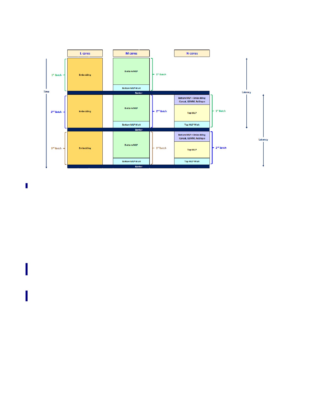
INTEL® ADVANCED MATRIX EXTENSIONS (INTEL® AMX)
Figure 20-23. A Recommendation System Multi-Threading Model
20.17 SPARSITY OPTIMIZATIONS FOR INTEL® AMX
This section describes how Intel AMX can be further optimized for operations on sparse matrices. An
example use case can be the inference of sparse neural networks, where the sparse weights are known
to initially reside in DRAM due to the “online” usage model or large model capacity. In those cases, the
primary performance bottleneck would be bringing the weights from DRAM. A helpful optimization tech-
nique for this case is to get the weights from DRAM in a compressed format, decompress them into the
local caches using Intel AVX-512, and perform Intel AMX computations on the decompressed data.
The compressed matrix format can consist of the following components:
• compressed[]: an array of non-zero matrix entries.
• mask[]: a bit-per-element array for the full matrix. 0 signifies the corresponding element is 0. 1
signifies a non-zero value that exists in the compressed[] array mentioned above.
The compressed format can be computed off-line. The sparsity bitmask mask[] can be generated using
the Intel AVX-512 VPTESTMB instruction on the sparse data. The compressed[] array can be generated
using the Intel AVX-512 VPCOMPRESS instruction on the sparse data using the sparsity bitmask.
20-55
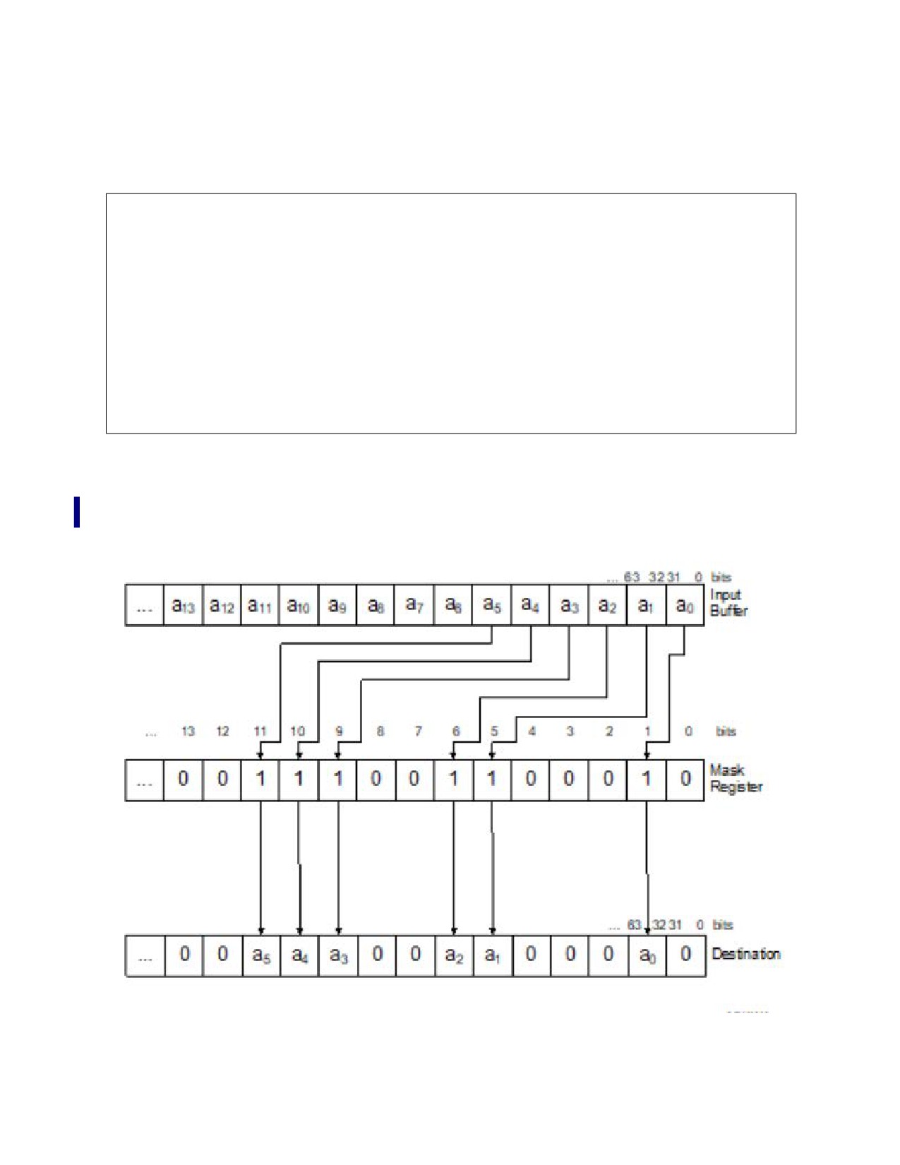
INTEL® ADVANCED MATRIX EXTENSIONS (INTEL® AMX)
The code in Example 20-27 uses Intel AVX-512 to generate num rows of decompressed data, assuming
8-bit elements and 64 elements per tile row.
Example 20-27. Byte Decompression Code with Intel® AVX-512 Intrinsics
// uint8_t* compressed_ptr is a pointer to compressed data array
// __mmask64* compression_masks_ptr is a pointer to bitmask array
// uint8_t* decompressed_ptr is a pointer to decompressed data array
for (int i=0; i < num ; i++) {
__m512i compressed = _mm512_loadu_epi32(compressed_ptr);
__mmask64 mask = _load_mask64(compression_masks_ptr);
__m512i decompressed_vec = _mm512_maskz_expand_epi8(mask, compressed);
_mm512_store_epi32(decompressed_ptr, decompressed_vec);
decompressed_ptr += 64; // 64 bytes per decompressed row
compressed_ptr += _mm_countbits_64(mask); // advance compressed pointer by number of non-zero elements
compression_masks_ptr ++; //64 bitmask bits per decompressed row
}
The matrix multiplication code will load the decompressed matrix to tiles from decompressed[], an
array containing the decompressed matrix data.
The decompression code makes use of the Intel AVX-512 date expand operation is shown in
Figure 20-24.
Figure 20-24. Data Expand Operation
20-56

INTEL® ADVANCED MATRIX EXTENSIONS (INTEL® AMX)
Decompression code for 16-byte elements can be designed in the same way.
For the best performance, apply the following optimizations:
• Interleaving: Fine-grained interleaving of decompression code and matrix multiplication to overlap
Intel AVX-512 decompression with Intel AMX computation.
• Decompress Early: Prepare the decompressed buffer before immediate Intel AMX use to avoid
store forwarding issues.
• Buffer Reuse: Decompressing the full sparse matrix could overflow the CPU caches. For best cache
reuse, it is recommended to have a decompressed buffer that can hold two decompressed panels of
the sparse matrix. While matrix is multiplying with one panel, decompress the next panel for the
subsequent iteration. In the subsequent iteration, decompress the next panel into the first half of the
decompressed buffer that is no longer used, and so on.
• Decompress Once: Coordinate the matrix multiplication blocking and loop structure with the
decompression scheme to minimize the number of times the same portion of the sparse matrix is
decompressed. For example, if the B-matrix is sparse, traversing the entire vertical M-dimension will
compress every vertical panel of the B-matrix only once.
20.18 TILECONFIG/TILERELEASE, CORE C-STATE, AND COMPILER ABI
For a function to use tile registers, it needs to configure them. For the LDTILECFG instruction definition,
see Section 20.2. LDTILECFG creates an Intel AMX state which is kept valid until the TILERELEASE
instruction is issued. TILERELEASE resets the Intel AMX state back to INIT. When the Intel AMX state is
valid, and the OS issues the MWAIT instruction trying to move the physical processor, it executes on to
Core C6 State. The 4th Generation Intel® Xeon® Scalable processor based on the Sapphire Rapids
microarchitecture will not enter Core C6 even if the sibling logical processor is idle. This is because it
lacks the dedicated backing store to keep the Intel AMX state until waking up. The Core C-State is
demoted to C1 instead.
This is not an issue in Linux and Windows, where only the idle process issues the MWAIT instruction. The
Idle Process in both operating systems does not use the Intel AMX ISA, so its Intel AMX tile state is
always invalid (INIT). If still valid, the Intel AMX tile state will have previously been saved in an OS-
defined area in memory while context-switching between a thread that uses Intel AMX and the Idle
Process thread.
20.18.1 ABI
The tile data registers (tmm0 - tmm7) are volatile. Their contents are passed back and forth between
functions through memory. No tile register is saved and restored by the callee. Tile configuration is also
volatile. The compiler saves and restores tile configuration and tile register contents if the register(s)
need to live across the function call. The compiler eliminates the save instruction because its content
remains the same on the stack. The compiler reuses the configured content saved on the stack before the
call. All functions need to configure the tile registers themselves; however, tile registers may not be
configured across functions.
Please download the System V Application Binary Interface: Intel386 Architecture Processor Supple-
ment, Version1.0.
20-57

INTEL® ADVANCED MATRIX EXTENSIONS (INTEL® AMX)
20.18.2 INTRINSICS
Example 20-28. Identification of Tile Shape Using Parameter m, n, k
typedef int _tile1024i __attribute__((__vector_size__(1024), __aligned__(64)));
_tile1024i _tile_loadd_internal(unsigned short m, unsigned short n, const void*base, __SIZE_TYPE__ stride);
_tile1024i _tile_loaddt1_internal(unsigned short m, uunsigned short n, const void*base, __SIZE_TYPE__ stride);
_tile1024i _tile_dpbssd_internal(unsigned short m, unsigned short n, unsigned short k, _tile1024i dst, _tile1024i
src1, _tile1024i src2);
_tile1024i _tile_dpbsud_internal(unsigned short m, unsigned short n, unsigned short k, _tile1024i dst, _tile1024i
src1, _tile1024i src2);
_tile1024i _tile_dpbusd_internal(unsigned short m, unsigned short n, unsigned short k, _tile1024i dst, _tile1024i
src1, _tile1024i src2);
_tile1024i _tile_dpbuud_internal(unsigned short m, unsigned short n, unsigned short k, _tile1024i dst, _tile1024i
src1, _tile1024i src2);
_tile1024i _tile_dpbf16ps_internal(unsigned short m, unsigned short n, unsigned short k, _tile1024i dst, _tile1024i
src1, _tile1024i src2);
void_tile_stored_internal(unsigned short m, unsigned short n, void*base, __SIZE_TYPE__ stride, _tile1024i tile);
The parameter m, n, k identifies the shape of the tile.
20-58

INTEL® ADVANCED MATRIX EXTENSIONS (INTEL® AMX)
20.18.3 USER INTERFACE
Example 20-29. Intel® AMX Intrinsics Header File
/* 1 of 2 */
typedef struct __tile1024i_str {
const unsigned short row;
const unsigned short col;
_tile1024i tile;
} __tile1024i;
/// Load tile rows from memory specified by "base" address and "stride" into
/// destination tile "dst".
///
/// \headerfile <immintrin.h>
///
/// This intrinsic corresponds to the <c> TILELOADD </c> instruction.
///
/// \param dst
/// A destination tile. Max size is 1024 Bytes.
/// \param base
/// A pointer to base address.
/// \param stride
/// The stride between the rows' data to be loaded in memory.
void __tile_loadd(__tile1024i *dst, const void *base, __SIZE_TYPE__ stride);
/// Load tile rows from memory specified by "base" address and "stride" into
/// destination tile "dst". This intrinsic provides a hint to the implementation
/// that the data will likely not be reused in the near future and the data
/// caching can be optimized accordingly.
///
/// \headerfile <immintrin.h>
///
/// This intrinsic corresponds to the <c> TILELOADDT1 </c> instruction.
///
/// \param dst
/// A destination tile. Max size is 1024 Bytes.
/// \param base
/// A pointer to base address.
/// \param stride
/// The stride between the rows' data to be loaded in memory.
void __tile_stream_loadd(__tile1024i* dst, const void* base, __SIZE_TYPE__ stride);
/// Compute dot-product of bytes in tiles with a source/destination accumulator.
/// Multiply groups of 4 adjacent pairs of signed 8-bit integers in src0 with
/// corresponding signed 8-bit integers in src1, producing 4 intermediate 32-bit
/// results. Sum these 4 results with the corresponding 32-bit integer in "dst",
/// and store the 32-bit result back to tile "dst".
///
/// \headerfile <immintrin.h>
///
20-59