Physics For Scientists And Engineers 6E - part 9

S E C T I O N   2 . 3     •     Acceleration

33

Conceptual Example 2.4 Graphical Relationships between x, v

x

, and a

x

(a)

(b)

(c)

x

t

 

F

t

 

E

t

 

D

t

 

C

t

 

B

t

 

A

t

 

F

t

 

E

t

 

D

t

 

C

t

 

B

t

t

 

A

O

t

O

t

O

t

 

F

t

 

E

t

 

B

t

 

A

v

 

x

a

 

x

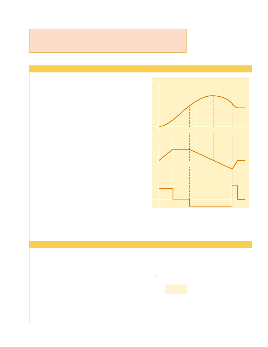
Figure 2.7 (Example 2.4) (a) Position–time graph for an ob-

ject moving along the x axis. (b) The velocity–time graph for

the object is obtained by measuring the slope of the

position–time graph at each instant. (c) The acceleration–time

graph for the object is obtained by measuring the slope of the

velocity–time graph at each instant.

The position of an object moving along the x axis varies with
time  as  in  Figure  2.7a.  Graph  the  velocity  versus  time  and
the acceleration versus time for the object.

Solution The  velocity  at  any  instant  is  the  slope  of  the
tangent to the x -t graph at that instant. Between t ! 0 and
t ! t

A

, the slope of the x -t graph increases uniformly, and

so the velocity increases linearly, as shown in Figure 2.7b.
Between t

A

and t

B

, the slope of the x -t graph is constant,

and  so  the  velocity  remains  constant.  At  t

D

,  the  slope  of

the x -t graph is zero, so the velocity is zero at that instant.
Between t

D

and t

E

, the slope of the x -t graph and thus the

velocity are negative and decrease uniformly in this inter-
val. In the interval t

E

to t

F

, the slope of the x-t graph is still

negative,  and  at  t

F

it  goes  to  zero.  Finally,  after  t

F

,  the

slope of the x -t graph is zero, meaning that the object is at
rest for t & t

F

.

The  acceleration  at  any  instant  is  the  slope  of  the  tan-

gent to the v

x

-t graph at that instant. The graph of accelera-

tion versus time for this object is shown in Figure 2.7c. The
acceleration  is  constant  and  positive  between  0  and  t

A

,

where  the  slope  of  the  v

x

-t graph  is  positive.  It  is  zero  be-

tween t

A

and t

B

and for t & t

F

because the slope of the v

x

-t

graph is zero at these times. It is negative between t

B

and t

E

because  the  slope  of  the  v

x

-t graph  is  negative  during  this 

interval.

Note that the sudden changes in acceleration shown in

Figure 2.7c are unphysical. Such instantaneous changes can-
not occur in reality.

Quick Quiz 2.3

Make a velocity–time graph for the car in Figure 2.1a. The

speed  limit  posted  on  the  road  sign  is  30 km/h.  True  or  false?  The  car  exceeds  the
speed limit at some time within the interval.

Therefore, the average acceleration in the specified time in-
terval $t ! t

B

#

t

A

!

2.0 s is

The  negative  sign  is  consistent  with  our  expectations—
namely, that the average acceleration, which is represented
by the slope of the line joining the initial and final points
on the velocity–time graph, is negative.

(B)

Determine the acceleration at t ! 2.0 s.

#

10 m/s

2

!

a

x

!

v

xf

#

v

xi

t

f

#

t

i

!

v

x

B

#

v

x

A

t

B

#

t

A

!

(20 # 40) m/s

(2.0 # 0) s

v

x

B

 

!

(40 # 5t

B

2

) m/s ! [40 # 5(2.0)

2

] m/s ! % 20 m/s

The  velocity  of  a  particle  moving  along  the  x axis  varies  in
time  according  to  the  expression  v

x

!

(40 # 5t

2

) m/s,

where t is in seconds.

(A)

Find the average acceleration in the time interval t ! 0

to t ! 2.0 s.

Solution Figure  2.8  is  a  v

x

-t graph  that  was  created  from

the  velocity  versus  time  expression  given  in  the  problem
statement. Because the slope of the entire v

x

-t curve is nega-

tive, we expect the acceleration to be negative.

We  find  the  velocities  at  t

i

!

t

A

!

0  and  t

f

!

t

B

!

2.0 s

by substituting these values of t into the expression for the
velocity:

v

x

A

 

!

(40 # 5t

A

2

) m/s ! [40 # 5(0)

2

] m/s ! % 40 m/s

Example 2.5 Average and Instantaneous Acceleration

So far we have evaluated the derivatives of a function by starting with the definition

of the function and then taking the limit of a specific ratio. If you are familiar with cal-
culus, you should recognize that there are specific rules for taking derivatives. These
rules, which are listed in Appendix B.6, enable us to evaluate derivatives quickly. For
instance, one rule tells us that the derivative of any constant is zero. As another exam-
ple, suppose x is proportional to some power of t, such as in the expression

x ! At

n

where A and n are constants. (This is a very common functional form.) The derivative
of x with respect to t is

Applying this rule to Example 2.5, in which v

x

!

40 # 5t

2

, we find that the accelera-

tion is a

x

! 

dv

x

/dt ! #10t .

2.4 Motion Diagrams

The concepts of velocity and acceleration are often confused with each other, but in
fact they are quite different quantities. It is instructive to use motion diagrams to de-
scribe the velocity and acceleration while an object is in motion.

A  stroboscopic photograph  of  a  moving  object  shows  several  images  of  the  object,

taken as the strobe light flashes at a constant rate. Figure 2.9 represents three sets of
strobe photographs of cars moving along a straight roadway in a single direction, from
left to right. The time intervals between flashes of the stroboscope are equal in each
part of the diagram. In order not to confuse the two vector quantities, we use red for
velocity  vectors  and  violet  for  acceleration  vectors  in  Figure  2.9.  The  vectors  are

dx

dt

!

nAt

n#1

34

C H A P T E R   2     •     Motion in One Dimension

10

–10

0

0

1

2

3

4

t(s)

v

x

(m/s)

20

30

40

–20

–30

Slope = –20 m/s

2

!

"

Figure 2.8 (Example 2.5) The velocity–time graph for a

particle moving along the x axis according to the expression

v

x

!

(40 # 5t

2

) m/s. The acceleration at t ! 2 s is equal to the

slope of the green tangent line at that time.

Solution The velocity at any time t is v

xi

!

(40 # 5t

2

) m/s

and the velocity at any later time t % $t is

Therefore, the change in velocity over the time interval $t is

Dividing this expression by $t and taking the limit of the re-
sult as $t approaches zero gives the acceleration at any time t:

Therefore, at t ! 2.0 s,

Because the velocity of the particle is positive and the accel-
eration is negative, the particle is slowing down.

Note that the answers to parts (A) and (B) are different.

The average acceleration in (A) is the slope of the blue line
in  Figure  2.8  connecting  points  ! and  ".  The  instanta-
neous  acceleration  in  (B)  is  the  slope  of  the  green  line
tangent to the curve at point ". Note also that the accelera-
tion is not constant in this example. Situations involving con-
stant acceleration are treated in Section 2.5.

#

20 m/s

2

a

x

!

(#10)(2.0) m/s

2

!

a

x

!

lim

$

t : 0

$

v

x

$

t

!

lim

$

t : 0

(#10t # 5$t) ! #10t

 

 m/s

2

$

v

x

!

v

xf

#

v

xi

!

[#10t 

 

$

t # 5($t)

2

] m/s

v

xf

!

40 # 5(t % $t)

2

!

40 # 5t

2

#

10t 

 

$

t # 5($t)

2

sketched at several instants during the motion of the object. Let us describe the mo-
tion of the car in each diagram.

In  Figure  2.9a,  the  images  of  the  car  are  equally  spaced,  showing  us  that  the  car

moves through the same displacement in each time interval. This is consistent with the
car moving with constant positive velocity and zero acceleration. We could model the car as a
particle and describe it as a particle moving with constant velocity.

In Figure 2.9b, the images become farther apart as time progresses. In this case, the

velocity vector increases in time because the car’s displacement between adjacent posi-
tions increases in time. This suggests that the car is moving with a positive velocity and a
positive acceleration. The velocity and acceleration are in the same direction. In terms of
our earlier force discussion, imagine a force pulling on the car in the same direction it
is moving—it speeds up.

In Figure 2.9c, we can tell that the car slows as it moves to the right because its dis-

placement between adjacent images decreases with time. In this case, this suggests that
the car moves to the right with a constant negative acceleration. The velocity vector de-
creases in time and eventually reaches zero. From this diagram we see that the acceler-
ation and velocity vectors are not in the same direction. The car is moving with a posi-
tive velocity but with a negative acceleration. (This type of motion is exhibited by a car that
skids to a stop after applying its brakes.) The velocity and acceleration are in opposite
directions. In terms of our earlier force discussion, imagine a force pulling on the car
opposite to the direction it is moving—it slows down.

The violet acceleration vectors in Figures 2.9b and 2.9c are all of the same length.

Thus,  these  diagrams  represent  motion  with  constant  acceleration.  This  is  an  impor-
tant type of motion that will be discussed in the next section.

S E C T I O N   2 . 4     •     Motion Diagrams

35

(a)

(b)

(c)

v

v

a

v

a

Active Figure 2.9 (a) Motion diagram for a car moving at constant velocity (zero

acceleration). (b) Motion diagram for a car whose constant acceleration is in the

direction of its velocity. The velocity vector at each instant is indicated by a red arrow,

and the constant acceleration by a violet arrow. (c) Motion diagram for a car whose

constant acceleration is in the direction opposite the velocity at each instant.

Quick Quiz 2.4

Which of the following is true? (a) If a car is traveling east-

ward, its acceleration is eastward. (b) If a car is slowing down, its acceleration must be
negative. (c) A particle with constant acceleration can never stop and stay stopped.

At the Active Figures link

at http://www.pse6.com, you

can select the constant

acceleration and initial velocity

of the car and observe pictorial

and graphical representations

of its motion.

2.5 One-Dimensional Motion with Constant 

Acceleration

If the acceleration of a particle varies in time, its motion can be complex and difficult to
analyze. However, a very common and simple type of one-dimensional motion is that in
which the acceleration is constant. When this is the case, the average acceleration 

over

any time interval is numerically equal to the instantaneous acceleration a

x

at any instant

within the interval, and the velocity changes at the same rate throughout the motion.

If we replace  by a

x

in Equation 2.6 and take t

i

!

0 and t

f

to be any later time t, we

find that

or

(2.9)

This powerful expression enables us to determine an object’s velocity at any time t if we
know the object’s initial velocity v

xi

and its (constant) acceleration a

x

. A velocity–time

graph for this constant-acceleration motion is shown in Figure 2.10b. The graph is a
straight line, the (constant) slope of which is the acceleration a

x

; this is consistent with

the fact that a

x

!

dv

x

/dt is a constant. Note that the slope is positive; this indicates a

positive  acceleration.  If  the  acceleration  were  negative,  then  the  slope  of  the  line  in
Figure 2.10b would be negative.

When  the  acceleration  is  constant,  the  graph  of  acceleration  versus  time  (Fig.

2.10c) is a straight line having a slope of zero.

Because velocity at constant acceleration varies linearly in time according to Equa-

tion  2.9,  we  can  express  the  average  velocity  in  any  time  interval  as  the  arithmetic
mean of the initial velocity v

xi

and the final velocity v

xf

:

(2.10)

Note  that  this  expression  for  average  velocity  applies  only in  situations  in  which  the
acceleration is constant.

We can now use Equations 2.1, 2.2, and 2.10 to obtain the position of an object as a

function of time. Recalling that $x in Equation 2.2 represents x

f

#

x

i

, and recognizing

that $t ! t

f

#

t

i

!

t # 0 ! t, we find

(2.11)

This equation provides the final position of the particle at time t in terms of the initial
and final velocities.

We can obtain another useful expression for the position of a particle moving with

constant acceleration by substituting Equation 2.9 into Equation 2.11:

(2.12)

This equation provides the final position of the particle at time t in terms of the initial
velocity and the acceleration.

The  position–time  graph  for  motion  at  constant  (positive)  acceleration  shown

in Figure  2.10a  is  obtained  from  Equation  2.12.  Note  that  the  curve  is  a  parabola.

x

f

!

x

i

%

v

xi

 

t %

1

2

 a

x

t

2

(for constant a

x

)

x

f

!

x

i

%

1

2

 [v

xi

%

(v

xi

%

a

x

t)]t

x

f

!

x

i

%

1

2

 

 (v

xi

%

v

xf

)t

   

(for constant a

x

)

x

f

#

x

i

!

vt !

1

2

 

(v

xi

%

v

xf

)t

 v

x

!

v

xi

%

v

xf

2

   

(for constant a

x

)

v

xf

!

v

xi

%

a

x

t

   

(for constant a

x

)

a

x

!

v

xf

#

v

xi

t # 0

a

x

a

x

(b)

v

x

v

xi

0

v

xf

t

v

xi

a

x

t

t

Slope  =  a

x

(a)

x

0

t

x

i

Slope = v

xi

t

(c)

a

x

0

a

x

t

Slope  =  0

Slope = v

xf

Active Figure 2.10 A particle

moving along the x axis with con-

stant acceleration a

x

; (a) the posi-

tion–time graph, (b) the

velocity–time graph, and (c) the

acceleration–time graph.

36

C H A P T E R   2     •     Motion in One Dimension

Position as a function of

velocity and time

Position as a function of time

At the Active Figures link

at http://www.pse6.com, you

can adjust the constant

acceleration and observe the

effect on the position and

velocity graphs.